
Figure 1: quartet card Vrouw en werk
Source: Volwassenen-educatie (Ov.)
The famous sociologist J.S. Coleman develops in his book Foundations of social theory a model of social exchange. In essence the model is based on the neoclassical theory of Walras, Jevons and Edgeworth. Coleman shows that she can be applied to social situations, beyond the economy. Then power replaces wealth. The present column discusses his formulas. Several fascinating cases are also elaborated, such as the occurrence of transaction costs or uncertainty. The column ends with illustrative examples.
The book Foundation of social theory by J.S. Coleman belongs to the sociological literature, but is nevertheless very relevant for economics1. Although the book is mainly written as a narrative, the fifth and final block (the chapters 25 until and including 34) contains a mathematical model of social actions. The present column wants to summarize the approach of Coleman in transforming the social interactions into abstract mathematical formulas. Here he uses the theory of marginal utility from micro-economics. Thanks to the theory of marginal utility the exchange of goods on the market by individuals can be described. Coleman has the original idea to apply this model to various forms of social exchange.
Coleman is interested in social phenomena, and these occur by definition at the macro level. However, he wants to explain the phenomena and events from the behaviour and actions of the separate individuals. The theory of marginal utility is suited for this, because her building blocks consist of separate subjects, who are just engaged in maximizing their utility, welfare and satisfaction. They try to maximize their utility by exchanging some of their possessions with other subjects. Those properties can be private goods, as well as a claim on the use of collective resources. These are means, that allow the actor i to exert power on others. For, other actors j desire the possessions of i. They are willing to make a concession in order to acquire them.
Now many human actions can be presented as a form of exchange between groups of persons. It is naturally great, when al those human actions could be calculated by means of a mathematical model. In order to avoid disappointment it is necessary to mention se at the beginning veral limitations of the model. Human behaviour is never merely based on the maximization of personal utility. The effect of the personal behaviour on other individuals is always taken into account. Furthermore, it is known from behavioural economics, that people dislike unjust treatment. They try to avoid that, even when thus some benefits must be given up. Moreover, the maximization of utility suggests a rational decision. However, the human cognition is by nature not tailored to be rational. There is a tendency to make misjudgements.
Several limitations of the micro-economic approach of Coleman are mentioned by Demeulenaere in his book Homo oeconomicus, which incidentally introduced your columnist to the work of Coleman2. Apparently the theory of exchange can not be applied in practice, and certainly not in the description of social events. Nevertheless, the exchange theory does improve the insight in daily life, because she illustrates the connection between social phenomena. As long as one realizes, that the model is an abstraction, there is much to learn. Therefore the approach has become popular, despite critics such as Demeulenaere. It is called the rational choice theory.
The exchange model of Coleman is a linear system of action. Your columnist has not encountered this approach in texts on economics. Evidently Coleman as a sociologists does not fear to posit a concrete functional relation for the individual utility function. Economists are reluctant to do this, because they want to free the theory from human morals. Suppose that in total M different types of goods are available. According to Coleman the satisfaction Ui of an actor i can be represented by the formula
(1) Ui(ci1, ci2, ..., ciM, t) = Σj=1M xji × ln(cij(t))
In the formula 1, cij(t) is the quantity of the good j, that the actor i possesses at the time t. The variable xji is a positive constant, which represents the desire of the actor i with respect to the good j. This becomes apparent when ∂Ui/∂cik is calculated, for the case of a fixed cij for j<>k. For, that is the change of utility due to a change in the quantity of the good k. The result is ∂Ui/∂cik = xki / cik. In short, according as xki increases, the utility grows more when the quantity of the good k expands. The result also shows, that the marginal utility is decreasing. In other words, according as cik increases, its desire saturates. In principle, xji could be measured simply by asking the actors about their preferences.
For loyal readers the formula 1 will not come as a surprise. For, already in 1931 the Dutchman Jacob van der Wijk introduces the formula U = κ × ln(x − m) for the utility of a quantity x of money. Here, m is a threshold value, and κ is a scaling factor, which is otherwise irrelevant, because other desires are omitted. Indeed it is commonly assumed, that the utility varies as the logarithm of the quantity of property. Thus in a column about the work of the Dutch economist B. van Praag it is assumed, that U = ln(Z) holds. Van Praag calls the variable Z the latent variable3. Therefore the formula 1 can be rewritten as
(2) Zi(ci1, ci2, ..., ciM, t) = ci1x1i × c21x2i × ... × cM1xMi
Loyal readers will also recognize the formula 2 from a column about the Hungarian economist M. Toms. However, he uses it for modelling the social target function Z, so as a policy instrument. It does not concern the individual needs. A function such as in the formula 2 is commonly classified as a Cobb-Douglas type, after the names of its inventors. However, Cobb and Douglas study a production function, and not a utility function. In Cobb-Douglas functions one often chooses Σj=1M xji = 1, so that the system is neutral with regard to scaling. Then the function is called linear-homogenous. However, Coleman makes the assumption Σj=1M xji = ξi, with ξi>0.
Now, Coleman considers the most elementary situation, where two actors (say I and II) will attempt to increase their personal utility by exchanging two goods j and k. In other words, I and II dispose of means (respectively cI,j and cI,k for I, and cII,j and cII,k for II), unfortunately none of them in the ideal proportion. This exchange problem can be solved with the method of the Edgeworth box. It is described in a previous column, so that henceforth your columnist assumes that it is known. In the Edgeworth box the iso-utility curves of I and II are combined in a single graph. A change can occur, when the iso-utility curves of I and II are tangent. In this manner, for a given initial state (cI,j(0), cI,k(0), cII,j(0), cII,k(0)) a contract curve can be constructed.
The method of the Edgeworth box does not impose a specific form on the utility function. Thanks to the extra assumption of Coleman, namely the formula 1, the contract curve can be calculated with the help of mathematics. For, on the contract curve the marginal rates of substitution MRS = -∂cij / ∂cik of I and II must be identical. Thus the calculated contract curve satisfies4
(3) xk,I × cI,j × xj,II × cII,k = xj,I × cI,k × xk,II × cII,j
Since the preferences xij are given as constants for both actors, the formula 3 can be drawn in the corresponding Edgeworth box. It is not in advance known where on the contract curve I and II will end. That is determined by the bargaining process, and possible institutional rules that impose limitations on the exchange, Although the exchange process itself occurs at the micro level, the institutional rules belong to the macro level. They are determined by the society.
Although the formula 3 expresses the behaviour of the contract curve, yet it gives little concrete information about the interactions between the actors in a social system. Therefore, now Coleman considers a perfect social system, which is the sociological equivalent of the economic market with perfect competition. Here all actors behave rationally, and their actions are not limited by institutions. Information is complete and available, so that no transaction costs are required for an agreement between actors. However, there is one difference with the economic market, namely that the available goods and therefore the events can possibly be indivisible. These are collective goods, which can in principle be claimed by everybody, and which can not be distributed on an individual basis.
The most well-known example is the natural environment, such as air, water and soil. These can be called public goods. A more daily example is the company car, which can be used by the personnel. Coleman mentions other examples, which are sometimes surprising (see p.47 and further in his book). In all these cases, finally such an agreement must be drafted, that a single person or organization has the ultimate say over the good or event. Thus in the system an exchange of partial rights can occur, that brings the indivisible good under the control of a certain actor or group of actors. When an actor disposes of a partial right of use, then he can attach a price or exchange value to it. Next he can decide to keep the partial right as his property, or to give it up in order to acquire another good.
It is obvious that precisely this social aspect makes the perfect social system so fascinating and intriguing. It truly deserves an analysis. However, the mentioned situation with two actors I and II is an exception. For, the society commonly consists of many actors. In the column about the Edgeworth box it has been explained, that in case of a large number N of actors the method with the Edgeworth box takes on a different form. It turns out, that the bargaining space rapidly decreases in size, according as more actors enter. When the number N of actors approaches infinity, then that space shrinks to a single point. In other words, then a unique competitive equilibrium has been created. Since in that system the individual actor can no longer bargain, there is a unique exchange ratio for any pair of goods.
The final situation is competely stable, because everybody must reconcile himself with the fixed ratio of exchange. The fixed exchange ratio coordinates the behaviour of the actors, as it were behind their backs. Therefore, according to Coleman the exchange ratio in the perfect system is a variable at the macro level. Nevertheless, this social system is not necessarily an economic market. Often it is not possible to assign a price in money to the private and indivisible goods. Therefore Coleman prefers to use the word value for such a good j, which he represents by the symbol vj. It is obvious that the absolute value of vj is meaningless. Relevant is merely the ratio, that is used in the exchange of two goods j and k. The number of units of the good j, that can be obtained for a unit of the good k, is given by the fraction vk/vj.
A particular value vj could be chosen as the so-called numéraire. That implies that the good of the numéraire has an absolute value of 1. However, Coleman fixes the absolute values of all goods in a different manner. Namely, consider the actor i, who at a time t=0 owns goods cij(0), with j=1, ..., M. The total of these resources has a value
(4) ri = Σj=1M vj × cij(0).
Coleman calls ri the power of the actor i. For, according as i owns more resources, he is better able to reward others. Since all actions are interpreted as a voluntary exchange, i will always keep the same value of resources and means. That is to say, ri is independent of time.

The total wealth of the system is Σi=1N ri. Define Σi=1N cik(0) = γk. This is the total quantity of the resource k in the system, which evidently also does not depend on time. Apparently one has
(5) Σi=1N ri = Σj=1M γj × vj
The total wealth in the system is evidently also conserved. Apparently the lefthand side does not depend on time. Now Coleman fixes the absolute value of the exchange values vj by equating the total wealth to 1. Note, that the total wealth is a variable at the macro level.
Thus the individual actor i must solve
(6) maximize Ui(ci1, ci2, ..., ciM, t), while having regard to the budget restriction ri
The quantities of the resources are the variables. Such a problem can be solved by means of the method of Lagrange. It uses the Lagrangian
(7) L = Ui + λ × (ri − Σj=1M vj × cij(t))
In the formula 7, λ is the multiplier of Lagrange. Suppose that the actor i reaches his optimum after a time t of exchange. Apparently in his optimum one must have
(8) Ui × xji / cij(t) = λ × vj
Since the formula 8 holds for all resources j in the optimum, each pair j and k in this equilibrium situation must satisfy
(9) xji / (vj × cij(t)) = xki / (vk × cik(t))
It is fascinating in the formula 9, that in the equilibrium state it describes the relation between the exchange value vj and the preferences xji of all actors (i=1, ..., N), assuming a given distribution cij(0). Coleman indeed shows, that in the competitive equilibrium a closed formula can be found for the exchange values vj. He starts with the scaling ξi of the preferences of the actors, and with their budget restrictions ri. These appear, when one slightly modifies the formula 9 and sums over j on both sides of the equation:
(10) vk × cik(t) × ξi = xki × Σj=1M vj × cij(t)
Modify the formula 10, and sum over i on both sides of the equation. Use the definition of γk, the total quantity of the resource k in the systen, then it follows that:6
(11) vk = (1/γk) × Σi=1N (xki / ξi) × Σj=1M vj × cij(0)
The formula 11 describes a set of M linear equations in vj. Since they all have vj=0 as a solution (with j=1, ..., M), apparently the formula 10 does not yet yield a unique solution. A unique solution (unequal to zero) does appear, when the mentioned scaling Σj=1M γj × vj = 1 is added. This indeed allows to calculate the vj for the competitive equilibrium.
Coleman shows that the formula 11, together with the scaling of vj, can be presented more succinctly in the matrix notation. First, note that vj represents a vertical vector v. In the same manner, cij(0) is an N×M matrix C, and xji is an M×N matrix X. Defin also two square matrices, where all elements are zero, apart from the diagonal, namely Γ = δkh × γk, and Ψ = δih / ξh. In these two formulas δhk is the well-known Kronecker delta, which is zero, except for h=k, where it is 1. Thus the formula 11 obtains the matrix form7
(12) Γ v = X Ψ C v
The formula 12 is a homogeneous matrix equation. The particular solution, which by definition is not zero, can also be formulated in the matrix form. First rewrite Σj=1M γj×vj = 1 in the form Σj=1M (Γ v)j = 1. Next define the M×M matrix Ε with elements εjk = 1/M, and the vertical vector η with elements ηj = 1/M. Thanks to these definitions the scaling can be written in the matrix form Ε Γ v = η 8. This matrix formula can be combined with the formula 12 in such a manner, that the result is (Γ − X Ψ C + Ε Γ) v = η. Thus the exchange value vector can be calculated directly from the matrix equation
(13) v = (Γ − X Ψ C + Ε Γ)-1 η
In the formula 13 the upper index (-1) implies, that the inverse of the matrix between brackets must be used. This completes the model. Since v is now known, the other important variables can also be calculated, such as the wealth r, and the matrix C*(t) in the competitive equilibrium. For instance, the formula 4 is in matrix notation r = C v.

In chapter 27 of his book Coleman gives several fascinating examples of the possible applications of the just presented perfect social system. They are discussed in the remainder of this column. First, the distribution of power among the actors is studied. The richess rI of the concrete actor I is the most general indicator of his power. For, he can use it to buy resources and partial rights of other actors. However, since this is a social system, and not purely an economic system, the exertion of power will not necessarily use money. Sometimes power is exerted, when I directly exchanges a resource j for a resource or partial right k of another actor II 9.
However, the actor II will sometimes not desire the resource j of I. Then the direct exchange fails. Nevertheless, the actor I can still acquire the resource k of II, namely by activating a third actor III. Then this actor III does need to desire the resource j of I. Moreover, III must have a resource, that the actor II is willing to exchange for his resource k. As a scheme this is I(j) → III → II, followed by I ← III ← II(k). The actor III has the role of intermediary. This is called an exchange of the first degree. Thus the direct exchange could also be called an indirect exchange of degree zero. This scheme can be expanded at will, for instance when also the indirect exchange of the first degree offers no solution. Then a fourth actor must be activated, for instance in the scheme I(j) → III → IV → II. That is an indirect exchange of the second degree. Etcetera.
The essence of this argument is that the actor I can control the actor II, even when I can not directly access II. In that case I must use his network. That control gets even stronger, according as the actors in the network of I do have power over II. Coleman even presents a quantitative elaboration of this mechanism. Your columnist summarizes his analysis with a few remarks in a footnote10.
In an imperfect system there will commonly be transaction costs, when two actors agree on an exchange of goods or resources. Transaction costs are a necessary evil and thus a loss, because they do not satisfy needs of the actors. Suppose that at the start the total wealth in the system equals 1, and that the realization of the social equilibrium requires a value rN+1 for transaction costs. Then in the equilibrium at the time t the total wealth will be reduced to Σi=1N ri(t) = 1 − rN+1.
Now Coleman extends his model of the social system with the loss in wealth due to transaction costs (see p.732 and further). Note that the formula 10 can be presented in matrix notation by v = Γ-1 X Ψ r(0). Insertion of r = C v leads to
(14) r(t) = C Γ-1 X Ψ r(0)
In the formalism from the discussion of the perfect system all wealth is conserved, so that r(t) = r(0) holds. This is no longer true for the case, where transaction losses occur.
For the sake of convenience define Z = C Γ-1 X Ψ. Then the formula 14 describes the relation ri(t) = Σh=1N zih × rh(0). This formula expresses that during the establishment of the equilibrium the actor i exchanges a part of his richess with the other N−1 actors. Suppose that αih is the efficiency of the exchange between i and h, with the αih values lying in the interval [0, 1]. Then the transaction losses can be incorporated in the model by modifying the formula into ri(t) = Σh=1N zih × αih × rh(0). Now, for the sake of convenience Coleman assumes that the power balances ri/rh do not change due to the transaction losses11. The richess of each actor falls with a fraction 1−rN+1, so that one has ri(t) = (1 − rN+1) × ri(0). Thus one finds ri(0) = Σh=1N zih × αih × rh(0) + rN+1 × ri(0).
Coleman wants to present also this formula in matrix form. The matrix Z can be replaced by the matrix Φ, with elements φih = zih × αih, with i and h in 1, ..., N. Moreover, he transforms Φ into an (N+1) × (N+1) matrix, by adding as its last column φi,N+1 = ri. For φN+1,N+1 the value 0 is chosen12. Then the lowest row becomes φN+1,h = 1 − Σi=1N zih × αih, for h < N+1. The reader can easily verify, that these definitions yield the result
(15) r(0) = Φ r(0)
In chapter 28 Coleman discusses an exciting theme, namely the role of trust in the social exchange. He notably analyzes the trust in the reliability of supply by actors. The starting point is that the exchange does not occur simultaneously. The actor i hands over some of his resources to the actor h, and the latter promises to compensate for his acquisition by delivering resources to the actor i at a later time. Since the supply of h to i is planned for the future, it is not completely sure. The actor i assumes, that the probability of supply is p. Thus there is a chain of three events: i supplies to h, h promises the supply to i with a probability p, and at the agreed moment h does or does not deliver to i. The actor i has control or power over his own supply to h, and over the bargain with h. However, he does not control the eventual supply.
The formula 1 illustrates the judgement, that the actor i must make. Suppose that i supplies the resource j to h, hoping to receive the resource k in return. His supply to h causes a lost utility of L = xji × ln(cij(t) / cij(0)). Note that cij(t) < cij(0) holds, so that L is indeed negative. The supply by h would yield a utility to i of G = xki × ln(cik(t) / cik(0)). Since this supply is uncertain, the expected utility is p×G. Apparently the actor i will agree to the transaction, when one has p×G + L > 0. Since p×G is less than G, the actor i will demand somewhat more of the resource k as a compensation, than in a situation where the exchange has a reliable supply. Note that due to the uncertainty it seems as though the interest coefficient xki transforms into xki' = p×xki. This modification also changes the interest sum ξi.
An exchange is always done between two actors. The actor h must also judge, whether the exchange is useful for him. Here several situations are conceivable. It is possible that h himself is convinced that he will deliver to i. In that case he will calculate his loss L under the assumption, that the delivery is certain. His judgement is not influenced by the actual uncertainty of the exchange. On the other hand, the situation is conceivable, that the actor h is also aware, that his delivery is uncertain. Then he can depreciate his loss, yielding p×L. Then it seems as though the interest coefficient equals xkh' = p×xkh 13.
The described transaction is an exchange for once. Coleman also considers the case, where the actor i assumes, that all supplies have a probability p of realization. He analysis this situation with the help of a marginal approach. The actor i uses the variable ∂Ui/∂cij in order to decide, whether he will exchange his resource j for the resource k. From the formula 1 it follows that one has
(16) ∂Ui / ∂cij = xji × Ui / cij + p × (xki × Ui / cik) × ∂cik / ∂cij
The first term in the right-hand side of the formula 16 expresses that the actor i loses due to the exchange. This is the marginal version of the term L. The second term expresses the expected profit p×G for this agreement. It contains the MRS of j and k.
Suppose that the vector v of exchange values is given. For, the actor i does not engage in transactions in a bilateral manner, but in a multilateral context. The vector v is truly determined at the macro level. Then the MRS must be identical to vj/vk. Now the actor i will be willing to give up the resource j, as long as a decrease of cij is accompanied by a rise of his utility Ui. That is to say, ∂Ui/∂cij < 0. He halts the exchange as soon as ∂Ui/∂cij = 0 holds. This is the equilibrium situation for the actor i. Insert this condition into the formula 16, then the result is
(17) xji × cik × vk = p × xki × cij × vj
This resembles the formula 9. Thanks to the formula 17 a better insight is obtained with regard to the effect of uncertainty on the exchange behaviour. Namely, note that an equal exchange occurs, so that in the equilibrium at the time t one must have cik(t) = (cij(0) − cij(t)) × vj/vk. Use the formula 17 to eliminate the variable cij(t), then the result is
(18) cik(t) = (vj/vk) × cij(0) × xki × p / (xji + xki×p)
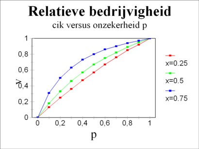
The question is interesting, what quantity cik(t) of the resource k the actor i wants to acquire, in comparison with the situation of guaranteed supply certainty p=1. Call this ratio ν. For the sake of convenience define ξi = xji + xki, then one finds for the ratio ν:
(19) ν = ξi × p / (ξi − xki × (1−p))
It is immediately clear, that ν rises according as the trust p increases. In other words, a society where the actors can rely on the honouring of agreements, furthers the trade and actitivies. According as the trust diminishes, the actors are inclined to keep their own property. The formula 19 also shows, that uncertainty can be compensated somewhat by desire. For, according as xki increases, the ratio ν will also rise. These both developments (p and xki) are depicted in the figure 4.
The present column is concluded with several examples of calculations, that have been copied form the book by Coleman, in a slightly modified form. The example merely serves to illustrate the various phenomena, and therefore is kept as simple as possible. Suppose that there are two actors, a farmer and an industrial producer. The farmer produces 10 bales of corn (cg,b = 10) during a period, and the manufacturer produces 10 machines (cm,i = 10) during the same period. The farmer wants to keep a part of his corn, among others for sowing, and he needs just a few machines. Therefore his column of interests equals xb = [0.8, 0.2]. The manufacturer can use the machines for himself, but he also needs corn in order to pay his workers. His column of interests equals xi = [0.5, 0.5]. The two columns together form the matrix X. The farmer and the manufacturer try to satisfy their needs by mutually exchanging bales of corn and machines.
Now, first calculations are done for this situation with the model of the perfect social system. Note that one has γb = γi = 10, and ξb = ξi = 1. The formula 13 is used for calculating the vector of values, resulting in v = (1/70) × [5, 2]. Apparently the ratio of exchange values is vg/vm = 5/2. Next with r = C v it is calculated, that the farmer has a power or control of rb = 5/7, and the manufacturer has a power of ri = 2/7. The ratio of the powers is 2.5. When the formula 9 is used, then after some calculations it is found that the farmer and the manufacturer exchange 2 bales of corn for 5 machines. Thus in the competitive equilibrium the farmer has c(t)b = [8, 5] and the manufacturer has c(t)i = [2, 5].
The following example concerns the same social system, however now with transaction costs. Suppose that the farmer and the manufacturer must both spend 5% of their richess in order to conclude the transaction. This means in terms of the developed notation that r3 = 0.05 holds. This situation occurs, when the farmer exchanges with an efficiency αb,m = 0.9, and the manufacturer exchanges with an efficiency αi,g = 0.75. The reader can easily varify, that thus the formula 15 is satisfied. For this simple case the matrix Z just equals the matrix X. Then the matrix Φ can be interpreted as a matrix of interests, where all coefficients are reduced due to the losses in the exchange, with the exception of those on the diagonal.
Coleman proposes on p.734 of his book to use the 2×2 sub-matrix in the upper-left corner of Φ as the interest matrix in the model of the perfect social system. When this is applied in the calculation with the formula 13, then one finds the result v = (1/100) × [7, 3]. The ratio of exchange values is vg/vm = 7/3. The farmer has a power of rb = 7/10, and the manufacturer has a power of ri = 3/10. Apparently, now the ratio of powers is 2.333, and thus it is slightly changed in favour of the manufacturer14. However, when the formula 9 is used again, then it turns out that merely 1.837 bales of corn have been exchanged for 4.286 machines. In this equilibrium the farmer has c(t)b = [8.163, 4.286] and the manufacturer has c(t)i = [1.837, 5.714]. So, due to the transaction costs the trade and activities are less than in the situation with perfect competition.
As a third and final example, here the social system with uncertainty is elaborated. The farmer supplies bales of corn to the manufacturer, but estimates that the probability of supply of the machines is merely p=0.7. The manufacturer has the sincere intention to deliver his products to the farmer. Thus the column of interests of the farmer changes into xb = [0.8, 0.14], whereas for the manufacturere it remains unchanged at xi = [0.5, 0.5]. The application of the formula 13 leads to the result v = (1/20) × [1.541, 0.459]. The ratio of exchange values is vg/vm = 3.357. The farmer has a power of rb = 0.77, and the manufacturer has a power of ri = 0.23.
Here the ratio of powers is 3.357, and thus the farmer is stronger than in the situation of total trust (p=1). This is a surprising find, which is also reported by Coleman (see p.751). When again the formula 9 is applied, then it turns out that merely 1.49 bales of corn are exchanged for 5 machines. In this equilibrium the farmer has c(t)b = [8.51, 5] and the manufacturer has c(t)i = [1.49, 5]. So due to the distrust the trade and activities are less than in the situation with complete certainty.