
Figure 1: plate ANMB
"Trouw aan de bond"
Many economic transactions have a time asymmetry, which forces the actors to trust each other. Trust is in the last resort built on a reputation. The present columns shows that actors signal their reputation to each other by choosing a certain behaviour. After a general introduction, based on the ideas of the sociologist J.S. Coleman, the signalling is illustrated with examples of the behaviour in oligopolies, of the policy of the central bank, and of applicants on the labour market.
Many columns in the Gazette have pointed to the imperfections of the neoclassical theory in her simplest form. These shortcomings are even felt to such an extent, that a new discipline has emerged, namely the behavioural economics. The behavioural economics rejects the image of man of the homo economicus, who in isolation tries, in a rational and egoistic manner, to enrich himself. For, the individual is embedded in the society, and accepts an extreme external control of his own behaviour. Thus the society can not be explained with a model, that presents the human interactions as impersonal exchanges of goods and means. The present column will show, that the personal reputation of individuals and organisations contributes significantly to their ability to succeed.
The sociologist J.S. Coleman has profoundly analyzed the behaviour in social interactions in his book Foundations of social theory1. For the remainder of the paragraph your columnist consults this rich source. Coleman states that the reputation affects the trust, that is given to the concerned person. Therefore he gives trust a central place in his discussion. Obviously the most interesting is that trust affects human actions. The approach of Coleman is characterized by a surprising ambiguity. Namely, on the one hand he sees man as a homo economicus, who rationally and purposefully tries to optimize his own welfare. And on the other had, that same man is again and again undermined by his own nature, including various urges, which seduce him into subjective and irrational behaviour2.
Trust is indispensable in human actions, because these are seldomly a direct exchange of goods and means. Often some time passes between the supply and the payment or service in return. The actor, who is the supplier in the transaction, makes an investment, as it were. The asymmetry in time is a risk for him, because it is uncertain, whether the actor, who is the recipient, will fulfil his obligation to pay. Apparently the supplier is a trustor, who gives trust to his buyer. Conversely, the recipient is a trustee, who is trusted. Often the trust will be granted thanks to the good reputation of the buyer. The supplier believes, that the chance of payment is high. Mathematically, this implies that p × Ow > (1 − p) × Qv. In this formula, Ow is the gain of the supplier in a successful transaction, and Ov is his loss, when the recipient breaks the trust and defaults3.
It would seem, that thanks to the conclusion of contracts the trust becomes dispensible. However, contracts are a deficient instrument. Often it is impossible to foresee all future developments. Sometimes the time will not allow the conclusion of a contract. More importantly, the conclusion of a contract causes extra costs, which reduce the profitability of the transaction and perhaps make her impossible. In short, the presence of trust furthers the activities. Therefore, the trust is sometimes called a social capital. In the simple neoclassical theory trust is superfluous, because she assumes that all individuals are completely informed. They perfectly know the situation of the other actors, and moreover are aware of all future developments.
It is clear that in the real world the actors dispose merely of incomplete information. They trust, that during a transaction the others do not supply false information or deceit in any other way. That trust can be formed as a consequence of the reputation of honesty of the other, which is based on the experience that his previous transactions have always been duly completed. Then this actor obtains a good name. This implies concretely, that the actor with a good reputation does not use deceit to enrich himself in the short run, for instance by defaulting on the payment. He prefers the gain, that he can obtain during future transactions with actors, who trust him. For, all actors, who must necessarily be trustors, will prefer a reliable trustee. Apparently the reliable actor trusts, that his buyers will remain loyal to him. Thus the relation is reciprocal.
It seems logical to interpret actions or transactions as economic activities. However, the argument can also be applied to other types of social activities. For instance, the politicians must continuously compromise with each other, and then often agreements are made for the long term. This can only succeed, when there is trust that the other will respect the compromise. A culture of trust is simply a collective ethics of the concerned group. This is not free and spontaneous. She must be formed gradually by investing in each other. Then a reputation is established, simply because one is included in the group. It will be clear, that the development of sound morals is complex. Namely, the aim is to diminish the costs of transactions, and nevertheless to maintain the mutual competition.
Breakers of the morals must be appropriately punished. The norm of sanctioning will first be informal, and later perhaps be laid down in a law, when the support is sufficient. The development of sound morals is a general interest. In this manner feed-back is included in the social system. On the one hand, the actor is restricted by the morals of his group. On the other hand, he is engaged in actions, which sometimes will change the system. Loyal readers will remember a particular case of this feed-back, namely the flows of information in a pluralistic democracy, as has been depicted in a previous column about the general interest. There the people are the trustor, and the government is the trustee. The system is society as a whole. It creates hope, that this system functions. For, a parliament and cabinet of purely homines economici would enrich itself without shame.
Some persons or organizations are intermediaries in trust. Coleman calls this behaviour entrepreneurial. The entrepreneurs bring together various investors in order to finance productive labour. In this model the workers are the trustees. But an entrepreneur can also bring together organizations, for instance in a cartel. The members of the cartel trust the initiator, and will later demand trust for themselves. Another example: the Central Bank has the goal to make the national currency trustworthy for the citizens. Reversely, the citizens rule the Central Bank, in the last resort.
When a large number of actors unite on the basis of mutual trust, Coleman calls this a group (see p.188). The group has a single goal and action, both aiming at the common interest of the group members. The group develops morals, and maintains these by means of sanctions, which in the last resort is the expulsion of the defectors from the group. The members of the group must obey their leader, for instance the entrepreneur, who has founded the group. Then the group turns into a hierarchy. The leader rises to power. There is a danger, that he leads the group astray, and then is corrected insufficiently or not at all by the members of the group.
Loyal readers will remember, that the Dutch economist P. Frijters repeats the arguments of Coleman in his book de An economic theory of greed, love, groups and networks4. He analyzes the reciprocal and hierarchical group, and in addition the network. A network consists of actors, who have mutual contacts, without agreeing on institutional norms. Frijters focuses his study on trade networks, where the entrepreneurs are the contact makers. Just like Coleman, Frijters takes the actor model of the homo economicus as his starting point. According as the trade network becomes more coherent, it can develop into a group. Each member of the group expresses his trust in the group by means of love. Thanks to his love that member himself is trusted by the remainder of the group. It is a risky strategy, because love has high costs5.
According to Frijters, love is not the same as trust. For, in the definition of Coleman the trust is calculated. However, love is an almost mythical process, which sometimes is even subconscious, and does not rely on external rewards (see p.87 in Aetoglgan). It is a complex of feelings and emotions. Therefore, on p.181 Frijters defines the trust as an embryonic form of love. Love stimulates the coordination of activities. In this manner a trade network can finally be seduced into establishing market institutions, which have the positive effect, that they diminish the transaction costs. Frijters even states, that in last resort the democracy has grown out of a market institution (see p.286, 304).
Apparently, in the elaboration of his theory he yet approaches the utility theory of Coleman. His objection to the theory of expected utility is, that it is not able to give a satisfactory explanation of group power (see p.219). Frijters also dislikes behavioural economics, because it has not yet developed a universal model. It is not able to describe society as a coherent system (p.222). In other words, Frijters desires to couple the micro-level to the macro-level. It has just been shown, that Coleman constructs the coupling by means of the influence of all individual actions on the system as a whole. The feedback to the macro system is realized at the micro-level. Just like Coleman, Frijters describes trust as a social capital (p.277). Trust can grow due to experience (p.278).
In short, Frijters adds the factor love to the explanation of Coleman. The homo economicus is by nature inclined to love. It enriches the social model with the inner drive of human bonding. Nevertheless, the proposal of Frijters has not yet been widely accepted in the scientific community. In the following several models will be explained, that illustrate the importance of a reputation. It concerns common models, where the concept of love is not yet introduced. Apparently it can be omitted here - although the models do not seem to exclude it. It concerns signals, which successively must suggest a strong monopoly, a strong Central Bank, and a highly productive worker.
In previous columns it has already been shown that the book Industrial organization in context by S. Martin is a goldmine for everybody, who wants to understand more about commercial organizations6. In the chapter 7 about dominant enterprises Martin describes two situations, where the enterprise benefits from signalling its "character" to its environment. In both situations the enterprise wants to signal its manner of setting product prices. The targets of the signals are respectively the buyers of the products and potential competitors on the market of the enterprise.
The first situation concerns the market of a durable product (see p.216). The enterprise introduces the product as an innovation, and therefore initially has a monopoly. A previous column has shown that in such a situation the monopoly can increase its profit thanks to price discrimination. Immediately after the market introduction the product price p(0) can be quite high, in order to sell to consumers with an excessive need. When that market segment is saturated, then in the next period t=1 the enterprise is tempted to lower the product price, say to p(1) < p(0). For, this will expand the market with consumers, who feel slightly less need for the product. Thus in subsequent periods t the price p(t) could be lowered in steps.
This policy is called a time inconsistency. It must be stressed that the enterprise is not malevolent in suggesting that p(0) is the right price. It simply concludes at t=1, that the welfare of the consumers can be improved by, on second thoughts, deviating from p(0). As long as the consumer indeed believes that p(0) is the right price, then everybody benefits from the new price policy. However, the new policy disregards, that each separate individual benefits from adapting his behaviour in the new situation. For, the falling price makes it advantageous for the consumers to wait with their purchase until later periods, even though they may agree with the present price. The consumer no longer believe the original price p(0). Therefore the famous economist Ronald Coase assumes, that the enterprise is forced to directly equate the product price to its marginal costs.
However, Coase suggests several signals to the enterprise, that can make the price p(0) credible. The enterprise can promise the consumers to buy back the product for the price p(0), reduced by a fair depreciation. When the consumer chooses this option, then he has actually rented the product. It is also possible to make slight changes to the product, in order to suggest that the original product has become obsolete. In that case the signal want to express, that the product is not particularly durable.
The second situation of signalling concerns a monopoly, that wants to discourage other enterprises from entering its market. Therefore the monopolist takes the initiative to produce a certain quantity Q. This model is called the Von Stackelberg type. It is supposed that the leader knows the best-reaction function of the entering enterprise. The demand curve is given by p(Q) = pmax − β×Q. For the sake of convenience, let the variable production costs of both enterprises by identical. Then in a previous column the mutual partition of the market is calculated. Let the initiator be I, and the new competitor be II. In an equilibrium on a shared market their productions would respectively be
(1a) qI = (pmax − c) / (2×β)
(1b) qII = ½ × qI
This formula can be used to derive a model of signalling, which is called limit pricing. This somewhat confusing term tries to express, that the monopoly I wants to limit the number of enterprises to just itself. It does not accept the partition of the market according to the set 1a-b. Therefore it must convince the enterprise II, that it will continue to suffer losses after entrance of the market. Concretely, I gives this signal by maintaining such a production capacity qI, that the price p(Q) can be lowered at will. When I nonetheless wants to remain profitable, then it must naturally keep its variable costs as low as possible. In the mentioned column it is shown that II can expect sales of
(2) qII = ½ × (pmax − c − β×qI) / β
Therefore the profit of II on the actual production is known as well, namely πII = (p(Q) − c) × qII. Insertion of Q = qI + qII and of the formula 2 yields
(3) πII = (½ − β/4) × (pmax − c − β×qI)²
Now, in this model it is assumed, that on entrance of the market II has fixed costs CII. When at a certain time the average capital efficiency equals r, and the yearly compensation to the owner of enterprise II equals πII, then the capitalized value equals πII/r. In other words, this is the capital value of the enterprise. Then the present discounted value of entrance equals
(4) WII = πII(qI) / r − CII
This formula clearly shows the power of I. For, according to the formulas 3 and 4, qI = (pmax − c) / β − (1/β) × √(r×CII / (½ − β/4)) will guarantee that WII=0 holds. A somewhat larger qI even implies an expected loss. Because of the demand curve, it is immediately clear, that the limit price for blocking the entrance of II equals
(5) p = c + √(r×CII / (½ − β/4))
The monopoly I must decide whether it wants to block. Blocking gives him a profit π1 = (p − c) × qI. Insertion of qI yields
(6) πI = (1/β) × √(r×CII / (½ − β/4)) × (pmax − c − √(r×CII / (½ − β/4)))
When the monopoly wants to make a rational decision, then it must compare this profit πI with the profit πI*, that results from allowing the entrance of II. Suppose still that it can lead with the quantity qI* (Von Stackelberg duopoly). From the formula πI* = (p − c) × qI*, from the demand curve and the set 1a-b it can simply be calculated that one has
(7) πI* = (pmax − c)² / (8×β)
Apparently I will block the entrance of II, if πI* < πI holds. Conversely, if πI* > πI holds, then I accepts the duopoly. The formula 6 shows clearly, that blocking becomes less attractive, according as the sunk costs CII are lower. A low rate of interest r can also be an obstacle for blocking.
Here the signalling towards II is done by means of the production capacity, which I has realized. Note that in the preceding argument it is assumed that both enterprises have identical variable costs c. However, when the entrepreneur II can reduce his costs (cII < cI), then he again makes blocking more difficult for I. Then the entrepreneur II needs to know the value of cI, and often that information will not be available. On p.225 of his book Martin considers the case of incomplete information for II, where however I does not know the best-reaction function of II. Since now I can not take the initiative, one has a normal Cournot duopoly. A market equilibrium is formed at qI = (pmax + cII − 2×cI) / (3×β), and qII = (pmax + cI − 2×cII) / (3×β). Then Q = (2×pmax − cI − cII) / (3×β) holds, and the profit of II becomes πII = (p − cII) × qII, so
(8) πII = (pmax + cI − 2×cII)² / (9×β)
The entrepreneur II will again employ the formula 4 for the present discounted value in order to calculate whether WII is positive. The formula 8 shows that the profitability depends both on the cost difference cI − cII and on the costs cII itself. Apparently the entrance is a gamble, as long as II does not know the value of cI. Now, II can make an estimate of cI by observing the production of I as a monopoly. Namely, in a previous column it is shown that the optimal production of the monopoly equals qIM = (pmax − cI) / (2×β). A monopoly with lower costs wil produce more than another with higher costs. It seems that II can yet obtain a reliable insight in the market.
A fully informed II is unpleasant for I, when its variable production costs are high. However, in that case a smart I will employ a trick. As a monopoly, it can make its production qIM larger than the optimum requires. In this way it signals to the entrepreneur II, that it has relatively low costs, lower than in reality. The monopoly masks its costs. Now, due to the formula 8, II will believe that he will make little profit after entrance on the market. Thanks to the mistaken illusion of II the monopoly I has in this way sent a discouraging signal to II. It is obvious, that I must beforehand calculate whether the deceit is profitable. On the one hand, this will perhaps ensure him that the monopoly on the market is maintained. On the other hand, as a monopoly, it produces too much, so that it loses a part of its profit. Signals to suggest strength actually occur quite often. The two following paragraphs also address this theme.
A previous column has shown, that the Central Bank benefits by influencing on each time t the expectations of the citizens with regard to the inflation πv(t). The theory of this macro-economic policy is explained clearly in the book Political economy in macroeconomics by A. Drazen, which is the main source for this paragraph7. The Central Bank (in short CB) is appointed by the state for stabilizing the prices. The furthering of the employment is mainly the task of the government, although the CB must also include it in its policy. The control of the expected inflation πv is important, because otherwise she will boost the inflation. An austere Central Bank (in short CB(A)) will not be troubled by πv, because the citizens know that it will always combat inflation. That is to say, it strives for π(t)=0.
On the other hand, a weak CB (in short CB(W)) has the reputation, that inflation is regularly tolerated, because it does not dare to oppose the government. For, the governement wants to combat the unemployment, and that creates some inflation. Therefore, the citizens distrust a promise by the CB(W) to engage in a policy with π(t)=0. The trust is absent. The CB(W) can influence πv merely, when and as long as it acts like a CB(A). Then the citizens are not certain about the type (A or W) of the CB. Here one recognizes from the preceding paragraph the masking by the monopoly with a large cI.
In the mentioned paragraph the loss function Λ(π, u) contains squares of the inflation π and the unemployment u. Here, Drazen prefers a somewhat different form, namely
(9) Λ(π, u) = μ × u(t) + π(t)²
In the formula 9, μ is a positive constant, which determines the value, that the CB attaches to the unemployment. The CB becomes more austere, according as its μ is smaller. Loyal readers know, that the CB wants to minimize its loss function. Except for unusual circumstances, u and π are mutually connected by the Phillips curve
(10) π(t) = πv − β × u(t)
For the sake of convenience, in the formula 10 the natural unemployment un is equated to zero. Now u is eliminated by inserting the formula 10 in the formula 9. The result is
(11) Λ(π(t), πv(t)) = (πv(t) − π(t)) × μ / β + π(t)²
The CB can obviously find the minimum of the loss function by calculating ∂Λ/∂π = 0. This yields the optimal πo = μ / (2×β). When the citizens base their expectation on this value, then the loss function becomes Λ = πo². It is striking, that the CB can obtain a better result by convincing the citizens, that they must assume πv=0. For, then Λ=0 becomes possible, by realizing π=0. It has just been concluded, that only a CB with an austere reputation can convince the citizens. Now Drazen wants to analyze how the reputation CB(A) can be created or maintained. He calls this the Backus-Driffill model of signalling. In this model the CB(A) chooses the inflation πo=πA, based on μA. It takes πA so small, that it approaches zero.
The model indeed distinguishes between two types for the CB, namely CB(A) and CB(W). Intermediate types are ignored. The CB(W) prefers π=πW with a relatively large πW, because its hallmark is a large μW. Mathematically formulated: πW >> πA. The development of the reputation is modelled by means of the calculus of probabilities. According to the citizens there is a probability p(t), that the CB belongs to the type CB(A). Suppose that the CB can indeed fully control the inflation. Then the CB can at a time t improve its reputation by choosing π(t) = πA. Suppose that there is a chance q(t), that the CB(W) indeed chooses this option in an attempt to improve its reputation. First, note that the citizens expect an inflation of
(12) πv(t) = (p(t) + (1 − p(t)) × q(t)) × πS + (1 − p(t)) × (1 − q(t)) × πZ
Apparently, at the time t two inflations are possible, namely πW and πA. The expected inflation πv(t) is located between these two values, as long as the citizens hesitate about the type of the CB. First suppose that in reality one has π(t)=πA. Then the so-called Bayesian rule can be calculated, that during the next period t+1 the citizens adapt their p in the following way:8
(13) p(t+1) = p(t) / (p(t) + (1 − p(t)) × q(t))
Since the denominator of the formula 1 is less than 1 (because less than p+1-p), one has that p(t+1) is larger than p(t). Apparently during the period t+1 the reputation of the CB is indeed improved. Next consider the reverse situation, where one has π(t)=πW. In other words, during the period t a significant inflation occurs. Then in a similar manner it can be shown that the adapted estimation equals9
(14) p(t+1) = 0
A large inflation proves to the citizens, that the CB belongs to the type CB(W). Henceforth it suffers from this reputation. The citizens will never again assume that πv = πA holds.
Furthermore, note that a far-seeing CB actually wants to minimize the loss function Λ = Σt=1ω δt-1 × Λ(π(t), πv(t)), where the symbol ω represents infinity. The factor δ discounts the future utility, which is felt less than the present utility. In other words, 0 ≤ δ ≤ 1 holds. Th CB obviously has a gigantic task, when it wants to derive the best available strategy for signalling from the optimization of Λ. Nevertheless, Drazen makes a serious attempt. Here he assumes that the CB is somewhat myopic, and merely considers the periods t=1 and t=2 10. In that situation, during the final period t=2 any CB, irrespective of its type, will choose its favourite inflation. That does not make a difference for the CB(A), because it always employs πA. However, the CB(W) will on t=2 prefer π(2) = πW. This gives it a weak reputation, but that merely affects the period t=3, which is beyond the time horizon of the CB.
In short, in this scenario the CB(W) chooses q(2)=0. Insertion in the formula 12 gives πv(2) = p(2) × πA + (1 − p(2)) × πZ. For the sake of convenience, rewrite for CB(W) the formula 11 as Λ(π(t), πv(t)) = 2×πW × (πv(t) − π(t)) + π(t)². Then one finds for the loss function of the CB(W)11
(15) Λ(π(1), p(2)) = 2×πW × (πv(1) − π(1)) + π(1)² + δ × (2×πW × p(2) × (πA − πW) + πW²)
Now the CB(W) will use the formula 15 in order to determine the signal with the smallest loss. A possible strategy is q(1)=0, where evidently CB(W) chooses π(1) = πW. Thus it reveals its type to the citizens, which results in p(2)=0. The loss function is simply Λ(πW, 0) = 2×πW × (πv(1) − πW) + πW² + δ × πW² = 2× πW × πv(1) − πW² + δ × πW². An alternative strategy is q(1)=1, which directly implies π(1)=πA. Note, that for this strategy with q(1)=1 a time inconsistency can occur, because CB(W) chooses q(2)=0. Nevertheless, in this model the citizens are sufficiently rational to know, that π(1)=πA does not mean that the type of the CB is A. The citizens still do not know the type of the CB. The formula 13 shows, that they judge the type according to p(t+1) = p(t), in casu p(2) = p(1). That yet creates consistency.
The essential question is which of the two options is most attractive for the CB(W). The formula for Λ(πA, p(2)) remains complex, but it can simply be calculated that one has12
(16) Λ(πA, p(2)) − Λ(πW, 0) = (πW − πA) × (πW − πA − 2×δ × πW × p(2))
(17) p(2) = ½ × (1 − πA/πW) / δ
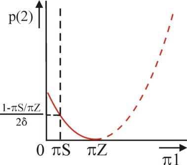
In short, the values of the discount δ, of the inflation difference πW − πA, and of the judgement p(2) = p(1) of the citizens determine the signal, that the CB(W) must send at t=1. When the formula 17 is satisfied, then both options q(1)=0 and q(1)=1 are located on the same iso-loss curve of Λ. In that situation the CB(W) could choose any arbitrary value of the probability q(1). Then its average chosen π(1) becomes q(1) × πA + (1 − q(1)) × πW. In this interpretation of π(1) as an average, π(1) in the formula 15 can apparently change continuously. In the figure 2 the corresponding iso-loss curve is drawn in the (π(1), p(2)) plane. It satisfies the formula p(2) = (π(1) − πW)² / (2×δ × πW × (πW − πA)) 13.
For the case that p(2) > ½×(1 − πA/πW) / δ holds, the CB(W) and CB(A) aparently choose identical strategies at t=1. This is called a pooling equilibrium. The CB(W) imitates the CB(A), at least at t=1. A CB with a large delta; will easily satisfy this requirement for p(2). For the case that p(2) < ½×(1 − πA/πW) / δ holds, the CB(W) and CB(A) apparently choose their own favourite strategy at t=1. This is called a separating equilibrium. The CB(W) immediately signals its type. In this situation δ will usually be small. However, note that δ has a lower boundary, because p(2) ≤ 1 must hold. That implies δ ≥ ½×(1 − πA/πW). When still the value of δ is below this boundary, then signalling is useless. The CB will simply choose its own preference, so that a separating equilibrium is formed.
The CB(A) does not need to choose its signals. However, it is hindered by the doubts p(t), that the citizens feel with regard to its type. For, according to the formula 12 this makes πv unnecessarily high. The formula 11 shows that thus the loss function increases. Fortunately there is a way out of this unpleasant situation, namely by keeping= πA as low as possible, for instance πA=0. Then the domain of p(2) values with a separating equilibrium is maximized, with p(2) < 1/(2×δ). When in this domain the separation π=πW does not occur, then the citizens can be sure that the bank has the CB(A) type. With this statement the explanation of the Backus-Driffill model can be concluded.
The preceding text exhibits impressive calculations, and Drazen wonders whether this is worthwhile. In fact the model was originally developed for describing signalling in oligopolies. Backus and Driffill have translated the model to the monetary policy, but a CB is naturally quite different from an oligopoly. Therefore the strategy of signalling will also be different. Nevertheless, your columnist believes that the Backus-Driffill model is worth the effort, because it illustrates some reactions of citizens, which must be taken into account by the CB. Therefore the model is presented here.
This paragraph analyzes the meaning of education for the economy. According to the theory of human capital the education supplies the citizens with extra knowledge and skills, so that they become more productive in their profession. However, this theory is rejected by scientists, who explain human skills by innate talents. These innate talents can be determined genetically, or they are transmitted during the formation, by the environment where one grows up. These scientists state, that education does not contribute to the productivity ap. The education is only useful, because it is a signal about the innate talent. Although this theory of signalling is intuitively odd, she has many adherents. The present paragraph explains her, by consulting chapter 12 in Microeconomic theory14.

The argument is as follows. Suppose that an individual, which has a productivity ap, experiences psychic costs c(e, ap), when he is educated for e years. For, commonly education is felt as a burden. In mathematical terms the yearly costs are C = ∂c/∂e > 0. These costs can partly be real, namely the tuition fee. Now make the essential assumption that people with talents excel in learning. Then for them the yearly costs are relatively low, notably the immaterial burden. In mathematical form: ∂C/∂ap < 0, or ∂²c/∂e ∂ap < 0 15. In other words, according as one's productivity is higher, the education becomes cheaper, and the individual will therefore be more willing to prolong his study. Exactly this personal property of studiousness makes his ap observable. It gives a signal, that is notably useful for entrepreneurs, searching for personnel.
The model divides the individuals in two groups, corresponding to their productivity, namely apL for the lowly-productive type L and apH for the highly-productive type H. This simplifies the analysis. Suppose that the society consists of N workers, and a fraction λ of them belongs to the type H. Apparently the average social productivity equals apG = λ×apH + (1 − λ)×apL. Then the society produces in total N×apG goods. The entrepreneurs can not distinguish between the two types, and therefore pay a wage w to everybody, in agreement with the average productivity. In other words, w = apG holds. Note that in this model the entrepreneurs do not make a profit.
Thus the entrepreneurs actually pay more to the type L than he is worth. Conversely, the type H is not rewarded according to his efforts. That irritates them. Now the type H has the finding to introduce an educational system. Then the education can signal the true value of H to the entrepreneurs. In a society with an educational system the individual utility function is
(18) u(w, v, e, ap) = w(ap) + v(ap) − c(e, ap)
In the formula 18, w is the wage that the entrepreneurs pay to the concerned individual. When the individual does not work, then he does not receive a wage. The variable v is the utility of an unemployed. Actually, this term is rather vague, because it contains several influences. It is true that the unemployment itself is a disutility, but on the other hand the unemployed benefit from the leisure time, from freedom and peace. Moreover, they can claim various benefits in money. Besides, it is conceivable, taht the unemployed start a business, and create an income from his independent activity. The variable v rather complicates matters, because in case of v>w the individual will reject working for wages. This is called the poverty trap. For now put v=0.
The formula 18 takes into account the signalling of ap. The type H can increase its utility, when the costs for his education are lower than the extra salary, that he will subsequently receive due to his apH. In this society with an educational system the individuals first select their education, and next the entrepreneurs offer a function with a corresponding wage. Here the entrepreneurs use a belief function μ(e), which expresses the probability that the type of the applicant is H. It has just been remarked, that the entrepreners believe in a positive correlation between μ and e. In short, ap(e) = μ×apH + (1 − μ)×apL. Thanks to the belief function and the formula 18 the labour market equilibrates. Microeconomic theory calls this a perfect Bayesian equilibrium (see p.452). Since the individuals and the entrepreneurs both make optimal choices, it is also called a Nash equilibrium.
The behaviour of the individuals can be derived by considering their iso-utility curves in the (e, w) plane: α = w(ap) − c(e, ap), where α has a fixed utility value. On the iso-utility curve ∂w/∂e = ∂c/∂e > 0 holds, that is to say, the curve is rising. Besides, the curve for the H type is somewhat flatter than the curve for the L type, because one has ∂C/∂ap < 0. This implies concretely, that the H type is willing to invest relatively much in education in order to increase his wage. That does not affect their utility (indifference). In the figure 4 these two iso-utility curves are depicted in the (e, w) plan, one for each type of individual. The two iso-utility curves intersect in exactly one point e=eo. When the education e lasts longer than eo, then the H type is satisfied with a lower wage than the L type.
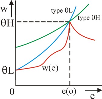
Next consider the behaviour of the entrepreneurs. Since they do not make a profit, they can offer a wage w = ap. The wage will be located in the interval apL ≤ w(e) ≤ apH. Lower wages are rejected by the workers, and higher wages would cause a loss. The offer of the entrepreneur is based on his belief function: e → μ(e) → ap(e) → w(e). It seems logical, that μ(e) and thus w(e) have a rising form, because signalling requires exactly this property. However, this is not necessarily true for all values of e. In Microeconomic theory several examples of w(e) are given, that are falling in some intervals of e. Your columnist has drawn such an equilibrium wage in the figure 4. It is clear that the two iso-utility curves have been chosen in such a manner, that they are tangent to w(e) in e=eo. There are obviously many more iso-utility curves for the types L and H, but merely these two are relevant for the present argument.
In the paragraph about the Central Bank it turned out, that signalling can lead to a pooling equilibrium or to a separating equilibrium. In the pooling equilibrium the entrepreneurs can still not distinguish between the types L and H. That state is just as irritating for the type H as the state where all have e=0. The type H clearly prefers a separating equilibrium. Fortunately for the type H a pooling equilibrium occurs merely for quite special wage curves w(e) 16. For the separating equilibrium the types L and H choose different durations of education. The entrepreneurs can distinguish between the two types, and pay L and H according to their effort respectively a wage apL en apH. Since according to the formula 18 the type L will suffer a loss of utility due to education at a given wage w = apL, it will prefer c=0, and therefore e=0. The type L foregoes education.
Apparently in the separating equilibrium the wage curve starts at w(0) = apL. For e>0, w(e) needs to remain below the iso-utility curve of L, because otherwise L would obtain an unnecessary wage rise. However, w(e) does need to reach its upper boundary apH somewhere in order to be able to hire the type H. That possibility occurs at e=eo, because there the iso-utility curve of the type L is "out of the picture". The type H wants to limit its educational costs, and therefore prefers that an iso-utility curve is tangent to w(e) exactly in this point e=eo 17. For the H type any e>eo causes additional educational costs, for an unaltered wage apH. This whole concurrence of desires results in the situation, that is depicted in the figure 4. Apparently the two signals for the L and H type are respectively e=0 and e=eo. It is true that in principle w(e) of the entrepreneurs can reach the upper boundary apH for an e>eo, but this equilibrium would not be socially optimal.
Note that the L type is worse off in a society with an educational system. For, the introduction of the educational system lowers their wage from an average of apG to apL. The H type is only better off, when λ < 1 − c/(apH − apL) holds18. When this threshold value of λ is exceeded, then the H type is also worse off in a system with signalling. For, when &lambda: approaches 1, then almost all individuals must educate themselves in order to distinguish themselves from the handful of L types. Then education creates gigantic social costs. Education could as well be omitted (e=0).
One would almost conclude, that signalling on the labour market is not such a good idea. However, the situation changes, when the formula 18 allows, that the utility v(ap) of unemployment is positive. Consider a situation without education and signalling. Then w will be equal to apG. Suppose furthermore, that for all ap the utility v(ap) is larger than apG, but less than apH. In that situation no individual is willing to work19. This situation will even occur, when an educational system does exist, but the equilibrium is pooling. For it has just been remarked that then everybody prefers e=0.
However, in this situation it turns out that a separating equilibrium does incite the H type to work, because now it can signal its type. For, this results in w = apH > v(apH). Since the H type obtains a higher income, now he is better off. In this separating equilibrium the L type gets offered a wage w = apL, and that is still less than v(apL) > apG. So the L type refuses to work, but it is not worse off than without signalling. Apparently the signalling now does improve the social welfare. That is due to the social security v. Thus it turns out that the conclusions of the model for signalling on the labour market depend strongly on the assumptions, that underly the argument20. Nevertheless, your columnist believes that despite this comment the idea of signalling yet adds an intriguing element to the understanding of the labour market.
The present column has analyzed signalling for three essential themes: the collusion in the industry, the devaluation of money, and the social importance of knowledge and skills. The foundation of the analysis is still the image of man as a rational, egoistic homo economicus. In these models a mutual sympathy, or a resistance against injustice, is strikingly absent. But the models do take into account the limits of human knowledge, and that is quite a step forwards in comparison with the old orthodoxy.
The models show that the human interactions at the micro level can truly be placed within a logical framework. Incidentally, the results of the models must not be taken too seriously, because they are largely determined by the preceding assumptions. Perhaps the utility of the models is mainly the effort, that is required to understand them. On the way one tends to discover that the assumptions of the theory are little more than a fairly extreme ideology.