
Figure 1: quartet card
Raiffeisenbank
Traditionally the monetary policy has been analyzed wit the AS-AD model. However, nowadays a new-Keynesian model is preferred, which is based on the Phillips curve and on the aggregated demand. The present column describes this model. Here, variants are also discussed, namely the Barro-Gordon model and a model with an infinite time horizon. The autonomy of the Central Bank is studied. It turns out that empirically the personal happiness is affected by inflation and unemployment.
In a previous column about economic planning the five most important policy goals are formulated. They are the curbing of unemployment, the stabilization of the prices, the equilibrated balance of payments, a just income distribution, and a durable economic growth. The state employs an ethics or morals in order to prioritize each of these goals. The policy is realized by means of policy measures, also called instruments. It is desirable that the contradiction between the various instruments is minimal. Therefore the state will design an economic plan, which guarantees the coordinated use of the instruments.
Of these five goals, the employment contributes most directly to the welfare of the citizens. Thanks to the theory of the Polish economist M. Kalecki and of the English economist J.M. Keynes, nowadays there exist instruments, which can significantly reduce the unemployment u. However, these instruments exert a negative influence on the other goals, notably on the inflation π. According as the unemployment u(t) decreases as a function of time, the price level P(t) tends to increase. Then the inflation, which is defined as π(t) = (∂P/∂t) / P, becomes positive. This negative correlation between u(t) and π(t) is formally expressed by the Phillips curve, where both variables are given as percentages. The unemployment percentage is measured as the number of unemployed with respect to the number of citizens, that is available on the labour market.
Recently in the Gazette a series of columns has been published, that explain how the preferences of the citizens are translated by the politicians into a concrete state policy. The ideas of politicians have a short time horizon, because they are motivated by successful elections. Therefore they are inclined to give a high priority to the reduction of unemployment. However, in the long term inflation can also be very damaging to the economy. For, unpredictable prices make it almost impossible to produce and trade in a rational manner. Therefore the stabilization of π must be pursued energetically. The politicians have safeguarded against the short-term pressure of the electorat by delegating the curbing of the inflation to an independent institute, namely the Central Bank (in short CB).
The Central Bank is responsible for the monetary policy. She supervises the quantity M of money of the state. This partly determines the price level P. For, suppose that the gross domestic product (in short GDP) is represented by Q, then P is proportional to M/Q. Thus the CB can exert some influence on the time development of π(t). Her policy affects u(t). This raises the ethical question whether the CB may back out of the democratic control process. In other words, the politicians must judge how much policy freedom (autonomy or independency) they want to give to the CB. Politicians vary greatly in their opinion, dependent on their ideology. The degree of CB autonomy is an essential theme of the remainder of this column.
This paragraph describes a new-Keynesian model, which explains the behaviour of the Central Bank. The model consists of three formulas, namely a formula for the Phillips curve, the formula for the economic demand(-function) and the formula for the lost utility of the CB. The Phillips curve is actually an empirical relation, and therefore many functions have been proposed to express her in parameters. In this paragraph your columnist follows the description in Grundzüge der Volkswirtschaftslehre by the German economist P. Bofinger, complemented with remarks from Macroeconomics by the American economist N.G. Mankiw1. Bofinger translates the Phillips curve into
(1) π(t) = πv(t) − gap(t) + f(u(t), un)
Although the formula 1 is originally empirical, yet she can be made credible with theoretical arguments. The term πv represents the expectation of the citizens with regard to the inflation. Namely, they will take into account the inflation, when making their wage demands and setting their product prices. Suppose that someone wants to sell his labour-power for a real wage wr. The inflation is a devaluation of money, so that the concerned supplier must be compensated by raising the value wr. When the worker expects that the inflation is πv, then the correction for inflation leads to πv×wr. In short, the expectation of the citizens with regard to the inflation creates a self-fulfilling prophecy, which raises the price level with πv.
However, a wage increase does not automatically generate inflation. For, at the time t the worker could become more productive than before. Suppose that his labour productivity ap(t) has a growth rate of gap(t), expressed in percents. Then his value-creating ability increases, and that makes a wage rise with this percentage realistic. Therefore gap must be subtracted, when calculating the inflation, in the manner of the formula 1. Note, that apparently the worker does not consciously add this increase in productivity to his wage demand.
The third term on the right-hand side of the formula 1 models the empirical correlation between π and u. The function f is decreasing with u, that is to say, she exhibits the behaviour ∂f/∂u < 0. The variable un is the natural unemployment. It occurs in the situation, where the production capacity of the industry is almost completely utilized. In many books, for instance also the one by Mankiw, the function f is made linear according to
(2) f(u(t), un) = -β × (u(t) − un)
In the formula 2, β is a positive constant. This implies for the case gap=0 that the natural unemployment is reached, as soon as one has π=πv. This suggests a kind of dynamic equilibrium, which explains the addition "natural". When moreover one has πv=0, then un becomes equal to the so-called NAIRU (in full non-accelerating inflation rate of unemployment).
Bofinger forgoes such arguments, and simply puts un=0. In other words, in the natural state there is full employment. In that state the GDP obtains the value Qn, and the corresponding national income is Yn = P×Qn. It is obvious that the unemployment will change, as soon as the actual national income Y(t) will deviate from Yn. The deviations in Y(t) are commonly expressed in terms of the relative output gap y, which is defined as
(3) y(t) = (Y(t) − Yn) / Yn
For the sake of convenience Bofinger assumes that one has f(u(t), un) = α×y(t), with α>0. In this manner yet a linear relation is introduced, albeit now between π and y 2. Furthermore, in the short term the productivity will be constant, so that gap=0 holds. And finally the possibility of an inflationary shock is taken into account by adding a term επ(t). All these remarks change the formula 1 into
(4) π(t) = πv(t) + α × y(t) + επ(t)
The formula 4 is the modified formula for the Phillips curve, which is the foundation of this model. The importance of the inflationary supply shock became clear after the two oil crises in 1973 and 1979, when the oil price suddenly jumped upwards. Since all activities require energy, such an increase of the price immediately affects the price level.
The second formula of the monetary model represents the aggregated demand function. As long as the savings S and the investments I are in equilibrium, the national income satisfies Y = C + I, where C is the total consumption. That is to say, there is a consumptive and productive demand. It is common to represent I by the investment function I = I0 − ι×r. Here I0 represents the autonomous investments, ι is een proportionality constant, and r is the real rate of interest. The consumption does not directly depend on r. Apply the formula 3, write y = (C + I − Yn) / Yn, and insert the investment function, then the result is3
(5) y(t) = η − ζ × r(t) + εy(t)
In the formula 5, η and ζ are constants. Besides, a demand shock εy(t) has been added, which serves to model the collapse of possible speculation bubbles.
The third formula of the monetary model is the utility function of the Central Bank. It is common to express the preference of the CB as a disutility or displeasure, following the early inventors of the utility analysis, such as Sam de Wolff. The CB is supposed to use a loss function, which is generally represented by
(6) L(π, u) = (π − πCB)² + μ × (u − uCB)²
In the formula 6, πCB is the inflation target of the CB, and μ is a non-negative constant. The formula shows, that the CB also has a target with regard to the unemployment. She tries to realize a level uCB. The size of μ determines the weight, that the CB attaches to this actually secondary target.
The quadratic form of L implies that the disutility will increase fast, according as π(t) and u(t) deviate more from their target values. In the optimum of the CB, L is made minimal, and therefore also the disutility and both deviations. When the CB prefers μ=0, then the unemployment does not interest her, and she supervises merely the inflation. Incidentally, Bofinger makes a somewhat different choice for the loss function than most other authors. Namely, he writes her as
(7) L(π, y) = (π − πCB)² + λ × (y − yCB)²
That is to say, here the CB tries to limit the output gap. Apparently, here Bofinger returns to the linear formula 2, which assumes proportionality for the deviations of u and y (with a negative sign)4. In that way the formulas 4 and 7 can both be drawn in the (y, π) plane.
The formulas 4, 5 and 7 express the various dependencies of the model. The inflation π can be removed from the formula 7 by means of the formula 4. Then the loss function only depends on y, so that the optimum of the CB is located in the point where ∂L/∂y = 0 holds. That optimum can simply be calculated5
(8) yo = (α×(πCB − πv − επ) + λ×yCB) / (α² + λ)
For the sake of convenience, Bofinger assumes, that the CB wants to mend the output gap (yCB=0).
It is clear that the results of the model will partly depend on the expectations πv, which are harboured by the citizens. That is intriguing, because apparently the human behaviour must also be modelled. As a start. Bofinger makes the logical assumption, that the citizens believe the policy targets of the CB. In that case they will choose πv(t) = πCB(t). Therefore the optimum of the CB has the compact form
(9) yo = -α×επ / (α² + λ)
It is striking, that the demand shock εy is not present in this formula. When the demand shock is not accompanied by an inflationary supply shock (επ=0), the CB can keep the output gap at y=0, so at its target value. Then, according to the formula 4, π also reaches its target value πCB = πv. The formula 5 gives the corresponding interest rate r = (η + εy) / ζ.
Unfortunately the CB can not reach her target point (yCB, πCB) = (0, πCB), when a supply shock occurs, perhaps in combination with a demand shock. The formula 9 shows, that the CB by necessity must tolerate an output gap. And the formula 4 shows, that the inflationary shock is merely tempered somewhat, to π = πCB + λ×επ / (α² + λ). According as λ is smaller, the inflation will approach πCB. But then at the same time the output gap would increase, and therefore the unemployment u. This clearly shows, that for a supply shock the curbing of inflation and unemployment can not be combined. For the sake of completeness, it must be mentioned, that according to the formula 5 the optimal interest rate is given by
(10) ro = (η + εy + επ×α / (α² + λ)) / ζ
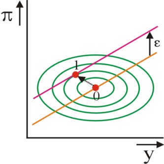
The case of the supply shock kan be conveniently illustrated graphically in the (y, π) plane. The figure 2 shows the original Phillips curve (0), in agreement with the formula 4, as well as the Phillips curve (1) after a positive shock επ. Also shown in the figure 2 are ellipses, that represent values of an equal disutility or loss. The starting point of the CB is the red dot on the right. After the shock the CB will attempt to keep her loss minimal, and therefore will choose as her optimum the point (yo, πo), where the iso-loss curve is just tangent to the new Phillips curve (red dot on the left). This point is reached by increasing the interest rate, so that the national income will shrink a bit. See the formula 10.
However, another situation can be conceived, namely when the Central Bank is not very credible. Incidentally, the failure of the CB to completely compensate the supply shocks can disappoint the citizens. In that case the citizens can give up their expectation πv = πCB. When the citizens act rationally, and moreover are completely informed, then they will estimate by themselves the reaction of the CB. They conclude that the CB chooses for the output gap yo of the formula 8. Next they insert that value in the formula 4 in order to obtain π(t). And that π also becomes their expectation πv. After some rewriting (with yCB=0) one finds the result6
(11) πv = πCB + λ × επ / α²
Apparently the rationally thinking citizens know, that the inflation will perhaps not become πCB. However, they have the problem, that the supply shocks επ(t) are commonly unpredicable. The prices can rise suddenly, but they can also fall suddenly. The citizens could simply assume, that the shocks occur statistically according to a normal distribution, with an average of zero. Then that average becomes the expectation value of επ(t). When this expectation is inserted in the formula 11, then the citizen yet finds πv = πCB 7.
A special case of the preceding situation occurs in the Barro-Gordon model. This model is explained in detail in Political economy in macroeconomics by the Israeli economist Drazen8. The model is usually formulated with the Phillips curve in terms of π and u, but your columnist again applies the formula 4 of Bofinger, with y as the variable. Barro and Gordon consider the situation, where the CB has an ambitious production target, with yCB>0. In other words, the CB wants to realize a positive output gap. In the optimum that gap equals the yo of the formule 8. Insertion of yo in the formula 4 gives the result
(12) π = (λ × (πv + επ) + α² × (πCB + yCB×λ/α)) / (α² + λ)
Again the actual inflation will depend on the behaviour of the citizens. Suppose first that the citizens are naive, and they expect that πv = πCB. In that case the formula 12 will reduce to
(13) π = πCB + (επ + α×yCB) × λ / (α² + λ)
In short, in the absence of a supply shock (επ=0) the inflation rises above the target value πCB. Suppose that this awakens the citizens, so that they begin to think rationally, and that they dispose of complete information. Now their expectation can again be calculated, just like previously for the formula 11. Therefore π in the formula 12 is equated to πv. Now the result becomes
(14) πv = πCB + yCB × λ/α + λ × επ / α²
Since supply shocks are unpredictable, for the sake of convenience the citizens will take επ=0. Therefore the last term on the right-hand side disappears. In this new situation π can be found by inserting the "rational" πv. When this expression is reformulated, then the right-hand side of the formula 14 is again obtained. In other words, on average one has π = πv. It turns out that the new expectation does agree with the actual development. The shocks will naturally still cause deviations, but this can not be remedied. Mathematically formulated: π − πv = επ × λ/α². When the shocks have a variance σ², then π will have a variance σ² × λ/α².
Summarizing, the policy of the CB causes an extra jump in the inflation of yCB × λ/α (called the bias). The formula 4 makes clear, that the well-meant attempt of the CB has a nasty consequence. For, due to the extra jump one has
(15) y = επ × (λ/α² − 1) / α
When shocks are absent, then y=0 holds. Apparently the CB yet did not succeed in reaching its target yCB>09! The unemployment remains identical to its natural value un, which belongs to the output gap of zero. This is somewhat problematic. Namely, the government will still be tempted to strive for yCB>0. For, this may succeed for a while, as long as the citizens are naive. A strong (independent) Central Bank is required in order to resist the temptation.
Interesting is also, that actually the citizens would benefit from being naive, instead of rational. For, as long as they stay naive, then the positive output gap remains present. Moreover, in this situation the inflation is lower than when all citizens begin to behave rationally10. Unfortunately, there is a conflict of interests. Each citizen clearly has the collective interest to believe the targets of the CB, but he or she also has the individual interest to estimate the inflation in an accurate manner. He needs this precise expectation in order to make sound wage demands, and in order to set the right price for his products. On p.120 of Political economy in macroeconomics such a conflict of interests is attributed to what Drazen calls the ex-post heterogenity. The individual differs from the masses.
It must be stressed that the administration does not malevolently give the impression that she strives for an inflation target of πCB. The administration simply concludes, that the welfare of the citizens can be improved by, on reflection, adapting the previously announced policy target. As long as the citizens indeed believe the original policy plans, then everybody benefits by the new policy. However, the new policy ignores, that each separate individual benefits from adapting his behaviour to the new situation. The policy volte face of the administration is called a time inconsistency. As soon as the citizens begin to adapt, the policy is again identical to their expectations, so that the consistency is re-established.
Strictly speaking the Central Bank not just wants to control the money stability at a time t, but also at all subsequent periods t+s, with s a positive integer number. Therefore, during the period t a prediction must be made about the future economic developments. Then a policy plan can be formulated for the long term. Here the CB can for instance accept somewhat more disutility during the period t, if thus the disutility in later periods can significantly be reduced. Such a model with an infinite time horizon is described in paragraph 4.2 of the book Politique économique11.
In each separate period t+s the loss function has the same form L(π(t+s), y(t+s)) of the formula 7, where for the sake of convenience the authors of Politique économique take πCB = yCB = 0. According as the disutility is located further in the future, it has less weight for the present, and therefore it is devalued with a factor δs (0 < δ < 1). The factor δ functions as a kind of discount for disutility. The loyal reader recognizes this approach from the previous column about behavioural economics. Furthermore, for all future periods (s>0) the loss function L(π, y) is based on a prediction, so that she can merely be an expectation. That is expressed by the notation Lv, where the lower index v refers to expectation. Thus the loss function Λ(t) with an infinite time horizon obtains the mathematical form
(16) Λ(t) = L(π(t), y(t)) + Σs=1ω δs × Lv(π(t+s), y(t+s))
In the formula 16 the symbol ω represents the value infinity. The model uses the Phillips curve of the formula 4. The aggregated demand function is again expressed like in the formula 5 12. Now note, that actually the formula 4 is a recursive relation. For, she can also by used for all periods t+s. Thanks to this iterative application of the formula 4 the end result becomes13
(17) π(t) = α × y(t) + επ(t) + Σs=1ω δs × (α × yv(t+s) + επ,v(t+s))
In the formula 17, yv(t+s) is the expectation of y(t+s) at time t, and επ,v(t+s) is the expectation of επ(t+s) at time t. Suppose that the CB can not influence the expectations with regard to π, y and επ. When now the CB searches her optimal Λ, then for her the sum-terms in the formulas 16 and 17 are merely constants. The requirements for the optimum is ∂Λ(t)/∂y(t) = 0. After some calculations one finds as the result again exactly the formula 9, which Bofinger has derived for the CB, when the future is not explicitly taken into account14. Nevertheless, the model with an infinite time horizon illustrates quite clearly, that it concerns truly rational expectations. They do not base on experiences in the past, or on promises, but on the infinite insight of the citizens in the future economic developments.
A discussion of the autonomy should really focus on the actual situation of the European Central Bank (in short ECB). However, there is so much literature about the ECB, that it merits a column of its own. Therefore, here your columnist restricts his arguments to the independency of The Dutch Bank (in short DNB), between 1967 and 1998. In this respect, the biographies of the two DNB directors from this period are relevant. J. Zijlstra describes his policy between 1967 and 1981 in Per slot van rekening, and the book Wim Duisenberg tells his adventures between 1981 and 199815. In the introduction of this column it has already been explained why it is desirable that DNB is independent of the government. Otherwise, the government could even force DNB to grant credits to the state. That would imply an uncontrollable creation of money.

Article 9 paragraph 1 of the then Banking Law states: "The Bank has the task to regulate the value of the Dutch currency in such a manner, as is required for the national welfare, and to stabilize that value as much as possible". Therefore DNB must make efforts to stabilize prices, but also to further economic growth. This corresponds to L(π y). Article 26 paragraph 1 is also important: "In those cases, where Our Minister [of Finance EB] believes it to be necessary for the coordination of the monetary and financial policy of the Government and the policy of the Bank, he gives instructions to the direction in order to realize that goal". In principle, this article makes DNB totally dependent on politics. However, it is merely intended to be an emergency measure, and therefore has never been used. Note that the Banking Law has been passed in 1948, when the general ambition was still a centralized, almost corporative, rule16.
On p.208 Zijlstra states that the article is useful, because it stimulates the deliberations between DNB and the minister. Incidentally, he calls DNB the ally of the minister of finance, who must curb the prodigality of his colleague-ministers (p.212). Zijlstra leads DNB precisely during the period, when the notion of the general interest and of social responsibility fade. The profitability of the Dutch economy collapses. After 1970 Zijlstra warns continuously against the unsound government policy, but the PvdA and even the CDA hardly listen17. It is obvious that the power of Zijlstra was quite limited, but yet in retrospect he reproaches himself that he has diminished the value of the currency too much (p.250).
At the time the trade union movement also criticizes the warnings of Zijlstra. On p.239 Zijlstra concludes in a resigned manner, that apparently this is its role18. Incidentally, Zijlstra has a good relationship with the social-democratic minister of finance Duisenberg, who finally will indeed succeed him. Duisenberg must experience the depression of 1981-1983 during his period as director. He attempts to make the guilder strong, and thus follows the same course as the centre-right cabinets under prime-minister Lubbers. More than Zijlstra, Duisenberg tries to couple the value of the guilder to the German Mark. Somehow this is curious, because this is also a loss of autonomy. Merely in 1983 the guilder is slightly devalued. According to his biographers, that is against the wish of Duisenberg, but he accepts the measure, because he believes that the policy of the exchange rate is the competency of the government (p.158).
In 1986 the European Act is signed, which sketches the path towards a single European currency. Since that moment the stability of the exchange rate becomes more important. Then Germany is the anchor state, that dictates a sound growth of the money quantity. Due to the coupling of the guilder and the Mark, DNB has hardly any policy freedom in the establishment of the interest rate. Incidentally, Duisenberg states that the short-term interest rate hardly influences the conjuncture, because the enterprises base their investments on the long-term interest rate (p.165). In 1995 the European stability- en growth-pact is signed. Thus, after 1985 the monetary policy becomes increasingly a European affair. The European Central Bank, which is founded in 1999, is mainly modelled with the German Federal Bank (Bundesbank) as an example. That is to say, she is completely autonomous, and must give the highest priority to price stability19.
Although the Central Bank disposes of freedom of policy, she is part of the state apparatus. Therefore she has the task to further the general interest, in casu the price stability, while having regard to the other policy targets. Therefore the loss function of the CB must be derived from the aggregated feelings of displeasure of the citizens. In chapter 6 of Happiness and economics various reasons are mentioned, that explain the dislike of inflation20. Contracts such as price lists and collective agreements are expressed in nominal sums of money. Inflation undermines the real spending power of the agreed wages. And it is not possible to continuously adapt the contracts to the reality. Therefore inflation introduces uncertainty about the real income of the citizens
Inflation leads to the devaluation of capital. The devaluation is commonly compensated by raising the interest rate as a price compensation. However, that forces the citizens to keep their capital in an interest-bearing form. They can not keep large sums of money in liquid form. Furthermore, the occurrence of inflation implies, that apparently the state has difficulties with the stabilization of the prices. Then the situation can easily get out of control, so that draconic measures will be needed in order to yet return to a stable currency value.

It is worthwhile to analyze the loss function of the CB also in this perspective. Therefore, consider its most simple form L(π, u) = π² + μ×u². On an iso-disutility curve one has that the marginal rate of substitution (in short MRS) of unemployment and inflation equals dπ/du = -μ × u/π. This can be rewritten as the elasticity η(u, π) = (∂π/∂u) / (π/u) = -μ × (u/π)². Apparently the loss function does not lead to a constant elasticity. According as π increases with respect to u, an bigger decrease of the unemployment is needed in order to compensate a given increase in π.
In Happiness and economics a reference is made to an empirical study about the dissatisfaction of citizens with regard to inflation. The dissatisfaction of the average citizen is modelled as21
(18) L(b) = -0.014 × π − 0.02 × u − 0.33 × ν(b) + ...
In the formula 18, ν(b) is a variable, which is 0 for workers and 1 for unemployed. It is immediately clear, that for the individual citizen the MRS(π, u) of the social unemployment and inflation is a constant, contrary to the just discussed judgment by the CB. The same holds for the MRS(π, ν) and the MRS(u, ν) with regard to the personal unemployment. Here a characteristic situation is observed, where the professional manager (in casu the Central Bank) prefers to make his own interpretation, and to not follow the preferences of the people.
If desired, the second and third term in the right-hand side of the formula 18 can be combined. That is to say, then one considers the disutility of the unemployed as a part of the social disutility due to u. For an average citizen a 1% rise of u implies, that the chance to become unemployed increases with 1%. That implies a statistical increase of his or her disutility with 0.0033. Then in the formula 18 the coefficient of u transforms into 0.0233. Thus one finds for the MRS(π, u) a value of 0.0233/0.014 = 1.66. In other words, when the unemployment u rises with 1%, then the inflation π must fall with 1.66% in order to conserve the disutility of the citizen. This exchange is true, independent of the height of π and u 22.
Note, that if desired the satisfaction of an income could also be added to the formula 18. According to p.114 of Happiness and economics that has indeed been done. An extra yearly income of $1000 turns out to diminish the disutility with 0.06. Apparently a 1% rise of the inflation causes as much disutility as a loss in income of $233. Here your columnist notes, that this kind of arguments must be seen as academic five-finger exercises, and are of a limited practical importance.
In the past it was common to explain the policy of the Central Bank by means of the AS-AD model. In the column about the AS-AD model its weaknesses have been extensively analyzed. The present column presents a new-keynesian model as an excellent and modern alternative for the AS-AD model. As far as your columnist can see, the new-keynesian model has none of the weaknesses of the AS-AD model. Moreover, in the new-keynesian model the preferences and the actions of the Central Bank and the citizens are better taken into account. Therefore it is a versatile model, that provides much insight in the economic interactions.
Unfortunately, this extension does not further the practical applicability of the theory. There is simply insufficient knowledge about human behaviour. A single example: there is no empirical justification for modelling the loss function of the Central Bank with the formulas 6 and 7. And sometimes the Phillips curve does not hold. She can be undermined by the adaptation of expectations or by rational expectations. Human behaviour is constantly changing. Your columnist accepts this. After all, one has to do something. What is truly desired, is a formal framework for ordering one's ideas. And here the model certainly succeeds.