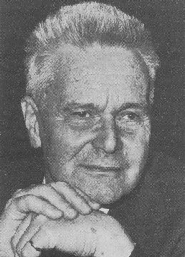
Figure 1: Jan Tinbergen
The well-known Dutch economist Jan Tinbergen develops in his book Economic policy: principles and design1 three simple models, which take into account the behaviour of the money market and of banking. The first model addresses the financing of the public sector, and the importance of the capital positions. In the second model the money- and capital-flows are traced, with special attention for the banks. The third model includes the central bank, so that the money creation is analyzed at the micro-economic level.

Tinbergen employs mathematical models, because they are useful in the analysis of the economic policy. A policy analysis starts with the formulation of the policy goals. An example of a general goal is the maintenance of the employment, and therefore the stabilization of the national income Y. The state disposes over certain instruments for realizing his policy. Such an instrument changes the value of one or more variables in such a manner, that finally the policy goals are approximated well. The relations of cause and effect are commonly represented by linear equations. The goals can only be reached, as long as the number of instruments is at least as large as the number of goals.
This type of models has been discussed before, for instance in the column about an open economy with variable prices, but there the influence of money and capital were ignored. The present column studies precisely this aspect. Three models are explained, where Tinberen has introduced monetary effects. The first model shows that wealth affects the expenditures of the households. The second model explains the role of banking in the control of the money- and capital-flows. The third model goes into the details of the operation of banking and the interaction with the central bank at the micro-economic level. The three models have in common, that the calculations of the national income Y take into account the circulation of the money quantity M and the trade B in bonds.
In this paragraph a model with two sectors is described, namely the private sector and the public sector2. The model intends to clarify how the state finances its expenditures. The foreign trade is ignored, which implies that the economic system is closed. The production of the two sectors is indicated by respectively XP and XG (G from the word government). The households earn their aggregate income Y thanks to the generation of the national product, so that one must have
(1) Y = XP + XG
The state disposes of three means to obtain money, namely the levying of taxes, the creation of money, and the borrowing from the households. Incidentally, the state can obtain money by selling state properties. The levying of taxes is presented by T = To + τ×Y. In this formula, To is the autonomous component of the tax, and τis the marginal tax rate. Money is created, when the state borrows directly from the central bank. For, the central bank is itself an institution of the state, so that the state borrows from itself - albeit with the obligation to later annihilate this extra money quantity by means of its redemption.
In this model Tinbergen puts B equal to the value sum of the shares and the government bonds. Thus both the issuing of the government bonds and the sale of state properties change the quantity B, which is owned by the households. Thus the state budget is given by
(2) XG = T + ΔM + ΔB
In the formula 2, ΔM is the creation of money, and ΔB is the income of the state from the sale of government stocks. The variables M and B are both a part of the capital, that is owned by the households. The consumptive behaviour of the households is modelled by the expenditure function
(3) XP = XPo(M, B) + ξ × Y
In the formula 2, XPo(M, B) is the autonomous component of expenditure. She depends on the capital position of the households, because these can eat into their capital, if desired. The variable ξ is the expenditure ratio of the households. Now the state wants to use this model in order to further the employment and stabilize the price level. In other words, Y and M must be controlled. Suppose that the desired national income is Y=YF (F for full, complete employment), and that the state wants to increase the money quantity with ΔMF. The size XG of the public expenditures and the size ΔB of the loans, concluded by the state, are used as the instruments. So the tax system, with parameters To and τ, remains unchanged.
The state, or the policy body which advises the state, can only solve the problem, when the autonomous component of expenditure XPo(M, B) is known. The simplest assumption is a linear dependency
(4) XPo(M, B) = η1 + η2 × ΔM + η3 × ΔB
In the formula 4 the parameters ηj are constant and positive. Apparently the pattern of expenditure of the households reacts to changes in the wealth3. Here the constant η1 does still depend on the initial conditions Mo and Bo of the quantities of money and government stocks. The formulas 1, 2, 3 and 4 allow to eliminate XPo and XP, which yields as result the values of the two instruments
(5a) ΔB = ((1 − ξ − τ) × YF − (1 + η2) × ΔMF − η1 − To) / (1 + η3)
(5b) XG = To + τ × YF + ΔMF + ΔB(YF, ΔMF)
First the size of the loan ΔB is calculated from the formula 5a. Since now ΔB is known, the desired size XG of the public product can also be calculated, with the formula 5b. In principle the set of equations 5a-b offers the state the possibility to curb the economic conjuncture, under an acceptable future inflation. On p.75 and further in his book Tinbergen pays attention to the market demand for bonds, emanating from the households. This subject has been discussed before in the column about the IS-LM model, which analyses the speculation part of the money demand. There the special case occurs, that the households must use all their money for their transactions, and thus almost empty their speculation cashes. In the present model XP represents the expenditures of the households, and therefore the transaction part of the money demand equals α×XP. The parameter alpha; is related to the circulation velocity of the money4.
In other words, when the speculation cash becomes empty, then the expenditures are no longer determined by the size of Y, but by the money quantity. For, the model assumes a stable price level. In the formula 3 one can put ξ=0, and XPo(M, B) takes on the form (Mo + ΔM) / α. The set of equations 5 changes into
(6a) ΔB = XG(YF, ΔMF) − To − τ × YF − ΔMF
(6b) XG = YF − (Mo + ΔMF) / α
First XG is calculated from the formula 6b. Then ΔB can be calculated from the formula 6a, which is simply the formula 2 in another form. Apparently there will still be a trade in government stocks, in spite of the almost empty speculation cash.
The reverse situation occurs, when the speculation cashes are well filled. Here Tinbergen refers to the situation at the end of a war, where the people were forced to save for a long time. At that moment the national production is low in comparison with the money quantity M. Therefore the state will try to reduce M, and he wants to raise Y. Now M can indeed be reduced by selling the government stocks to the households, at least if the households are willing to do so. However, it is conceivable, that the households are not interested, for instance because the rate of interest is too low (the so-called liquidity trap). In that case the state has no other choice than to introduce a new currency. Tinbergen calls this the monetary purge.
The discussed model supports notably the policy for state expenditures, but ignores the financial sector. Therefore Tinbergen has developed yet another model, where the capital flows are calculated explicitely5. Contrary to the previous model, which explains mainly the causal relations, here the formulas are mainly based on book-keeping. Yet also this approach contributes to the insight. Since the financial sector is pre-eminently international (even then!), the foreign states are included in the model. In other words, now the economic system is open. Thus there are three sectors, namely the national economy with the exception of the banks, the national banking, and the foreign states. The national income is given by
(7) Y = X + E − I
In the formula 7, X is the national product, E is the export, and I is the import. Tinbergen commonly assumes, that I/Y = ι is a constant. The wealth consists of money M (Tinbergen calls it liquid assets, so probably M3) and of government stocks (bonds). The matrix mij represents the money, which originates from the sector i and is now owned by the sector j. The sector i distributes a total money quantity of Mi = Σj=13 mij. In the same manner the trade in government stocks can be summarized by the variables bij and Bj. It is obvious that the sector 1 (national economy with the exception of the banks) does not create money, which implies M1=0. Neither does banking create government stocks, which implies B2=0.
The variable m3j is the inflow of money from abroad, where Tinbergen expresses the quantity in foreign currency. Therefore the exchange rate pw with respect to the national currency affects the domestic value of the money m3j, which originates from abroad. It is obvious that the government stock also has a price, namely p1 for the inflow b1j in the sectors j, and p3 for the inflow b3j in the sectors j. The prices are determined by the currency markets, the money market and the capital market.
Tinbergen defines the supply function of the national money by ΔM2 = Φ2(Y, p1, p3, pw). The supply function of the foreign money depends on the export, and is therefore slightly different: ΔM3 = Φ2(E, p1, p3, pw). The supply function of the foreing government stocks is ΔB3 = Ψ3(E, p1, p3, pw). The supply of domestic government stocks is a policy instrument, because the state can issue his own bonds. In other words, in this model ΔB1 can not be interpreted as an independent supply function.
On the demand side for money and government stock Tinbergen assumes, that the demand depends on the prosperity in the sector. The wealth in the sector can be written as
(8) Wj = p1 × b1j + p3 × b3j + m2j + (1/pw) × m3j
Note that W3 of the foreign states is expressed here in the national currency. Besides, Tinbergen assumes that the demand in a sector j is proportional to the money quantity m2j, which is owned by the sector6. Thus the demand in the sector j for foreign currency is determined by the function m3j = φ3j(Wj, p1, p3, pw) × m2j. And the demand in the sector j for government stock is determined by the function bij = ψij(Wj, p1, p3, pw) × m2j.
The behaviour on the markets determines the market prices p1, p3 and pw, and the quantities, which the participants in the three sectors want to own. In particular, now the expenditure function of the households can be stated7
(9) X = Xo + ξ × Y + η1 × p1 × b11 + η2 × p3 × b31 + η3 × m21 + η4 × (1/pw) × m31
The first and the second term at the left-hand side of the equation are supposed to be known. The following terms represent the wealth W1 of the households, where apparently Tinbergen expects different rates of expenditure ηk, depending on the nature of the wealth.
The model is completed with three formulas for financing. First, the domestic wealth will change, when the national income is not in an equilibrium with the national production:
(10) Y − X = p1 × (Δb11 − ΔB1) + p3 × Δb31 + Δm21 + (1/pw) × Δm31
In short, everything which flows into the sector 1, increases the income, and everything which flows out, decreases it. Second, the wealth abroad will change, when the import I to the state is not in equilibrium with the export E. Note, that here I represents the export of the foreign states, and E their import. The corresponding formula is
(11) I − E = p1 × Δb13 + p3 × (Δb31 − ΔB3) + Δm23 + (1/pw) × (Δm33 − ΔM3)
Third, the wealth changes under the influence of the balance of payments D. The balance of payments is the sum of the current account and the financial account8. Now, contrary to several previous columns it is no longer sufficient to calculate the trade balance and the terms of trade. The surplus or the deficit on the balance of payments is now given by9
(12) D = I − E − p1 × Δb13 + p3 × Δb31
Tinbergen recommends the presented model for policy analyses with regard to the full employment YF and an equilibrated balance of payments DF. These two policy goals can be realized by using two instruments: the expenditures Xo and the debt policy ΔB1. For, the state influences Xo by means of his own expenditures. And he can change B1 due to the trade in government stock. When for instance more is imported than exported, then the state can raise the rate of interest on its bonds. This will increase the sales of bonds to the foreign states. It depends evidently on the foreign demand Δb13 whether this will indeed equilibrate the balance of payments. In any case it is merely a temporary solution. In the long term I = E must truly be satisfied.
The third model of Tinbergen describes the interaction between the central bank and banking10. Contrary to the two preceding models, here the micro-economic phenomena are addressed. Perhaps the most interesting aspect of this model is the insight in the way of fixing the rate of interest. So the system of the second model is extended with the central bank, in addition to the three mentioned sectors. Now the operation of banking is elaborated. Each bank has the claims GB (in account current, short-term savings, and short-term deposits elsewhere) and the reserves R at the central bank on the debit side of her balance. On the credit side of the balans are the deposits MB and the rediscount GC at the central bank11. The balans is in equilibirium when one has
(13) MB + GC = GB + R
Probably the term rediscount requires a further explanation (which incidentally Tinbergen omits). When the bank wants to dispose of extra money, then she sells bills of exchange to the central bank. Bills of exchange can not immediately be transformed into liquidity, and therefore the central bank corrects the value of the bill for the lost interest. This is called the rediscount of the bill, and the applied rate of interest is called the precentage of discount12. Tinbergen uses the symbol rC for the rate of discount of the central bank. The central bank expresses the momentary value of possessing liquidity by means of the value of rC. These are costs for the banks, which are naturally passed on in the actual rate of interest on the money market.
The central bank has GC on the debit side of her balance, as well as the value Au of her stocks in gold. On the credit side of her balance are the money quantity M and the reserves of the banks13. The balance is in equilibrium, when one has
(14) M + R = Au + GC
Next Tinbergen presents a set of empirical linear equations, which allow to calculate the variables in the formulas 13 and 14. The Bretton Woods system requires that the ratio Au/M is larger than a certain constant σ. In the same manner, the central bank obligates the banks to keep the ratio R/MB above a certain constant ρ. Thus a logical formula for the rate of discount is
(15) rC = η1 + η2 × (σ × M − Au)
The formula 15 suggests that the rate of discount can be reduced, when the stocks of gold rise above the Bretton Woods requirement. She can be called the supply equation of credit by the central bank. In the same manner the supply equation of credit by banking can be expressed as
(16) r = ξ1 + ξ2 × (ρ × MB − R)
Tinbergen defines r as the particular rate of discount, which the banks earn on their deposits GB. For the sake of convenience, but perhaps misleading, this may be called the rate of interest. The banks will increase the number of rediscounts, according as it becomes cheaper and more can be earned by them. In formula this is
(17) GC = ξ3 + ξ4 × (r − rC)
The remaining empirical equations first require the calculation of the national income. Here Tinbergen employs the formula
(18) Y = ε1 + ε2 × Xo − ε3 × r
In the formula 18, Xo represents the autonomous national expenditure. The dependency on r in the formula resembles Y(r) in the commodity sphere of the IS-LM model. Now the demand on the money market can be represented by
(19) M = ε4 + ε5 × Y − ε6 × rC
The formula 19 is naturally exactly the money demand, which is found in the monetary sphere of the IS-LM model. It is composed of a transaction part and a speculation part. Here, Tinbergen has replaced the rate of interest by the rate of discount, because M is the money creation by the central bank (chartal money). In the same manner, the demand for deposits is given by
(20) MB = ε7 + ε8 × Y − ε9 × r
Finally, the balance of trade is given by
(21) I − E = ξ5 × ΔrC − ξ6 × ΔAu
The variables ΔrC and ΔAu are the changes, that occur during a period Δt (for instance a year). These additions give a dynamic character to the model. The formula 21 illustrates a phenomenon, which can also be observed in the second model, namely that a deficit on the balance of trade must be compensated by an increase of the rate of interest. In that situation the central bank can also decide to sell a part of her gold stocks. The national income inters in the formula 21 due to the relation I = ι×Y. This completes the model.
Tinbergen suggests ways to apply the model for policy analyses. Suppose that the state adheres to the goal of full employment, which requires a certain national income YF. Suppose that the state also has the goal of an equilibrated balance of payments. The formula 18 shows that r must be controlled, and for this rC is a convenient instrument. The formula 16 shows, that the requirement ρ of the banks is an alternative instrument for this. First note, that the choice of rC as the policy instrument means, that the formula 15 becomes irrelevant. Note furthermore, that due to the formula 21 the goal of the equilibrated balance of payments can be translated into the desire for a certain size of the gold stock Au. In other words, this goal can be reformulated as Au = AuF. Indeed it appears from the formulas 13-21, that with the right choice of rC and ρ the goals YF and AuF can be realized14.