
Figure 1: Telephone card Tinbergen
Since the beginning this portal has presented many models for calculations of the macroeconomic national dynamics. The present column addresses two themes, which were not yet discussed, namely the influence of the prices and the influence of the foreign trade. It is true that the price system has been explained by the theory of Sraffa, but she is hardly capable of modelling dynamical behaviour. The Dutch economist Jan Tinbergen has made several proposals to extend the Harrod-Domar model with a price effect. It is worth while to repeat his ideas here.
The inclusion of the foreign trade is essential for the modelling of a state, that disposes of an open economy. For then the global influences affect the domestic relations. Often such a state is not autark (able to satisfy its own needs), but it is forced to import certain goods. Then one has an international division of labour. The state benefits most from the foreign exchange, when it specializes in those types of production, where it is pre-eminently conpetitive. The comparative advantage of the state is expressed by the relatively low costs of production.
In such cases the domestic price of the product lies below the price on the world market. The product can be sold on the world market at a surplus profit. In theory the state could specialize completely in the production of a few such goods. In practice this situation never occurs, because there are additional costs of transportation, when goods are trades abroad. Besides, even on the world market the demand for a product is never unlimited. Therefore some diversification of the national production will always be required1.
In the book Mathematical models of economic growth Tinbergen includes the variable prices and the foreign trade in his multi-sector model2. The multi-sector model is discussed in a previous column, but yet it will be explained succinctly here. Let the economic system have N productive branches, each with a production volume of Qn (n=1, ..., N). Each branch n supplies his product to the other branches m, where they are consumed during the production as production factors, with a quantity of qnm. Moreover, the branch n supplies his goods to the branch m for its investments, with a quantity of jnm. It is obvious, that also a part of the product Qn serves to satisfy the domestic consumption Cn. Then the residue is available for the export
(1) En = Qn − Cn − Σm=1N (qnm + jnm)
In the formula 1 En is the difference of the export and the import. In other words, when more is consumed than produced, then a quantity -En must be imported. In that situation En is negative. As usual in Mathematical models of economic growth, Tinbergen defines the investment function by
(2) jnm = κnm × (Qm(t + θ) − Qm(t)) / θ
The variable θ is the period, which passes between the investment of the branch m and the coming into operation of the investment. The matrix κnm is the "partial" capital-coefficient. The total investments are
(3) I = Σn=1N pn × Σm=1N jnm
In the formula 3 pn is the piece price of the product, which is generated by the branch n. Thus the variables in the formule 1 are indeed quantities, and their value must be determined separately by the multiplication with the product price. In the mentioned previous column about the multi-sector model this is not the case. There the prices are simply pn=1, so that the quantities are identical to their values.
The price vector p appears also in the formula for the national income
(4) Y = Σn=1N pn × (Qn − Σm=1N qnm) = Σn=1N pn × (Qn − Σm=1N anm × Qm)
In the right=hand side of the formula 4 the production coefficients anm = qnm / Qm are inserted. In this way a simple vector notation Y = p · (I − A) · Q can be employed, where I is the unity matrix and the matrix A has elements anm. That notation makes sense only, when the anm do not depend on Qm.
The savings S are again calculated from the national income by means of the savings quote σ = S/Y. Here σ is independent of Y, and of the time t. Furthermore, the model assumes a balanced growth with S=I. The consumption is C = Y-S. Tinbergen again chooses the well-known consumption function, however now with the inclusion of a price effect
(5) pn × Cn = γn × C + pn × Γn + Σm=1N γnm × pm
In the formula 5 the γn are the marginal propensities to consume for the product n, and Γn is its autonomous consumption. The extra term with the "partial" propensities to consume γnm must guarantee, that the autonomous consumption is influenced by price changes in the other branches.
An interesting aspect of the model is the dynamic response of the product price pn to the product volume Qn. This is a striking difference with the theory of Sraffa, which describes a system in a market equilibrium. For, here the policy maker wants to make an optimal use of his comparative competitive advantage, and therefore he wants to supply as much as possible of his product speciality on the world market. However, that supply will push down the global product price, depending on the price elasticity of the demand. In short, one has pn = pn(Qn).
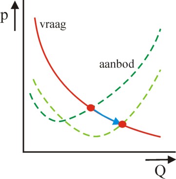
According to Tinbergen the situation gets more complex, when the state distinguishes between the domestic prices and the prices on the world market3. Also it would be necessary to take into account the substitution between products. Besides, the possible scaling effects are a second cause of the dependency pn(Qn) between the product price and the production volume. Those scaling effects refer to the cost function of the production. For, in the market equilibrium the demand curve intersects with the supply curve, which represents the costs. Demand and supply together determine the price. The is illustrated in a graphical manner in the figure 2, with two cost functions, belonging to different scales of production.
In the application of this model it can be imagined, that the policy maker is confronted with a given production Q(0) at the time t=0. Then the product prices pn(Q(0)) are also given. A simple one-sector model has already been employed in order to choose a certain savings quote σ. Therefore a monetary sum S(0) = σ × Y(0) can be invested. The challenge for the policy maker is to reach a maximal national income Y(θ) at the end of the investment period θ, starting from the monetary budget S(0). He or she will have to analyze all possible production options Q(θ),
In mathematics this is called the problem of Lagrange. It requires for the time θ the solution of the set of equations
(6) ∂Y / ∂Qn + λ × ∂S(0) / ∂Qn = 0
The parameter λ in the formula 6 is called the multiplier of Lagrange. Note that Qn(θ) appears in the formula of S(0) because of S=I and the formulas 2 and 3. Unfortunately Tinbergen ends his argument precisely at this point, where it gets exciting. Nevertheless the preceding text gives already a fair impression of the problems of policy makers, and of the way to solve them.
In Mathematical models of economic growth the presented model is notably recommended for the policy development with regard to the foreign trade. For a developing economy the import of certain vital products is indeed a necessary condition. And that import is only possible, when the necessary foreign currencies are obtained by means of export. The trade balance Σn=1N En must be at least equilibrated. Nevertheless it is clear - although Tinbergen does not state this explicitely -, that really the planning for the domestic market must take into account the price effects as well.
The model in the preceding paragraph is useful for analyzing the desired development of the economic structure. It is however rather cumbersome. Often a simpler model will do for the policy maker, and it can even give deeper insights. Suppose for instance, that the central planning agency wants to maximize the future national income Y, under the conditions of a full capacity utilization of the capital, an equilibrated trade balance, and a given savings quote4.

The model describes an open economy. Tinbergen treats the foreigns states as a single branch, and therefore calls this model a two-sector model. In fact it is a simple one-sector model of the Harrod-Domar type, with as the fundamental equations S = σ×Y, S=I, I = ∂K/∂t. and K = κ × Q. Note that here a distinction is made between the national income Y and the national (physical) product Q. The aim of the model is to calculate the conditions (terms of trade), which limit the foreign trade of a state. This requires the division of the trade surpluses En in de export volume EXn and the import volume IMn. Since the model has a single sector, one has n=N=1.
Suppose that the export has an average price pEX(EX), and the import has an average price pIM(IM). It is obvious that the product prices again exhibit the behaviour of the figure 2, depending on the price elasticities of the demand. The price behaviour of EX and IM is different, because the composition of the sets of goods is different. Notably the developing states sometimes have a one-sided export assortment of raw materials (oil, gas, minerals, agricultural products like coffee or suger cane, etcetera), whereas their import often consists of capital goods. It is obvious that the state benefits from a maximal ratio π = pEX(EX) / pIM(IM) 5.
The difference between the national income Y and the national product becomes apparent, when their balances are compared:
(7a) Q = C + I + EX − IM
(7b) Y = C + I + pEX × EX − pIM × IM
The expression in the formula 7b looks a bit sloppy, because C and I do not contain their prices. Apparently here for the sake of convenience pC = pI = 1 is assumed, where these prices are about equal to the general domestic price index. The price index is the numéraire for the export- and import prices, as it where.
The equilibrated trade balance is characterized by pEX × EX = pIM × IM, that is to say, by π×EX = IM. For a given pIM one has EX = EX(π), where the price elasticity of the demand EX is defined as ε = (∂EX / ∂π) / (EX / π). Under normal circumstances ε will be negative. Assume for the sake of convenience, that the elasticity ε does not depend on EX, then one has EX = η × πε, where η represents the value of EX for π=1. Finally, define the import quote ι as IM/Q. With all these relations one finds after some cumbersome calculations the time behaviour of the price ratio π: 6
(8) π(t) = (π(0) - β) × eα×t + β
For the sake of convenience, in the formula 8 the definitions α = (σ/κ) × (1+ι) / (1+ε) and β = ι / (1+ι) are used. This shows that apparently for ε>-1 the price ratio is more favourable, according as the time passes. In that case the terms of trade become better and better. However, when one has ε<-1, then the future looks gloomy.
In all its simplicity the model is ingenious. Thus from IM=ι×Q and EX=η×πε it can be concluded that Q = (η/ι) ×π1+ε. This can be combined with the relation Y = (κ/σ) × ∂Q/∂t. For, the policy maker can now determine, which savings quote yields the optimal national income. That requires ∂Y/∂σ = 0, and due to the cited relations and the formula 8 this requires ∂π/∂σ = 0. That leads to the condition ∂(α × t)/∂σ = 0, and thus to α×t = constant, so that apparently the savings quote must fall with the inverse proportion of time!
In his later book Economic policy: principles and design Tinbergen adds refinements to the described model7. This makes them more realistic and more generally applicable. Therefore the formalism, which is described in Economic policy: principles and design, is probably already quite close to the methods, which are applied by central planning agencies. The seamy side of the approach is, that due to the increased complexity analytical solutions of the formulas no longer exist. The models must be solved numerically.
A difference with the set 7a-b is, that no explicit distinction is made between the consumption C and the investments I. These two variables are simply merged in the real domestic expenditures B. The expenditure function is introduced in place of the investment- and consumption functions
(9) p × B = γ1 × Y + β + γ2 × p
In the formula 9 p is the domestic price level. The parameter γ1 is the marginal propensity to expend. The autonomous expenditures have a "nominal" component β and a price-dependent component γ2×p. The parameter γ2 is called the price coefficient of the expenditures. It shows what the households really want to expend in any case, physically, and it obviously depends on the price elasticity of the demand.
In this approach the real domestic product equals Q = B + EX. Another difference with the preceding paragraph is that the export price pEX may deviate from the price pW of the export goods on the world market. The formula EX = η × πε remains valid, but here π represents now the ratio pEX / pW. The import is coupled to the import-quote ι = IM/Q. Furthermore, a deficit on the trade balance is allowed:
(10) D = pEX × EX − pIM × IM

Perhaps the most important difference with the model of the preceding paragraph is the precision, with which the present model calculates the prices. Thus the domestic price level is obtained from the formula8
(11) p = p0 × QτQ × pLτL × pIMτIM
The formula 11 has the form of an extended Cobb-Douglas function. The variable pL is the price of the factor labour, that is to say, the domestic wage level. The coefficients τQ, τL, and τIM depend on the various price elasticities. For, the behaviour of the producers determines, to what extent the costs of production are imposed on the consumers. The quantity p0 is simply a constant of proportionality.
In a similar manner the export price is modelled
(12) pEX = pEX,0 × QρQ × pLρL × pIMρIM × pWρW
The coefficients ρQ, ρL, and ρIM differ from the coefficients the formula 11. Besides, in the formula 12 the world market price appears, with as coefficient ρW.
There exist certain dependencies between the coefficients and the various variables in the model9. For instance, it can be supposed, that ρQ and τQ approximately equal Q / (Q + IM), and are thus inversely proportional to 1+ι. For, according as the import becomes more important, the influence of the domestic production on p and pEX diminishes. In the same way ρIM and τIM will be approximately proportional to IM / (Q+IM), and thus proportional to ι / (1+ι). Furthermore Tinbergen assumes, that ε and EX are proportional10.
There is also a dependency of the coefficients due to the time horizon11. When a certain variable changes its value, then in the short run this will exert influence mainly on one other variable. But in the long run the change will exert more influence, because with some lag also the other variables will be affected by the change. Suppose for instance that the wage level rises. According to the formulas 11 and 12 that directly affects p and pEX, with the coefficients τL and ρL as weights. However, in the long run the tariffs of the independent workers will rise with the wages, so that p and pEX increase once more. The model takes this into account by using larger values of τL and ρL for the long run.
Readers who are interested in the formulas of the model for the macro-economic variables, such as Y, Q, D and p, are encouraged to consult p.106 and further in Economic policy: principles and design. Tinbergen consults econometric studies in order to determine the values of the various elasticities and coefficients. Unfortunately such data are not very accurate, and that makes the model subjective. Moreover, the formulas 11 and 12 are extreme simplifications of reality. For instance, it would be desirable to identify those export branches, which are truly affected by the changing wage level, etcetera12. These marginal notes show, that the economic policy is and remains the responsibility of politicians, and not of economics.