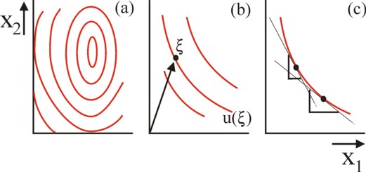
Figure 1: fields of indifference curves: (a) a complete field;
(b) field around the point ξ ; (c) MRS in 2 points on the same curve
The theory of the individual utility functions allows to model the operation of the competitive market. In particular it can be proven, that the competitive equilibrium really exists, provided that certain conditions are satisfied. This model can be clarified by using the so-called Edgeworth box, a rectangle which represents a bilateral market. Thus it can be shown that the individual preferences finally lead to a market price, so that all markets are cleared completely.
The aim of this column is to explain the exchange process by means of the Edgeworth box. In principle this is a subject, which can be found in any introductory textbook about micro-economics. However it is striking, that often the explanation is incomplete, and thus may cause misunderstandings. Therefore it is worthwhile to elaborate on the subject in the present column. Moreover, this column can become the starting- and reference-point for more advanced discussions in future columns.
The Edgeworth box uses the fields of indifference curves of individuals or of separate households. In various columns the phenomenon of iso-utility or indifference curves has already been explained. Figure 1a shows once more the field for an individual in a graphical manner. It allows to determine the quantities x1 and x2 of two goods, which as a whole have the same utility for the individual. In most textbooks it is assumed, that the utility continues to grow, according as x1 and x2 increase. This assumption is obviously not realistic. In reality there will always be a point of saturation. That is to say, the field of indifference curves describes a utility mountain1, and not a utility slope. This phenomenon is shown in the figure 1a.
In the real world the individual clearly never knows all his preferences. Usually his personal preferences are closely related to the actual situation of the individual, or to his past experiences. He can not imagine other needs - or he has never reflected on them. In other words, the indivudal knows merely the indifference curves around the quantities ξ1 and ξ2, which are in his possession. Note, thay this can be represented by a vector ξ in two dimensions. Furthermore, the application of the Edgeworth box requires, that the indifference curves exhibit a monotonous behaviour. They must be convex. In fact this implies, that the situation under consideration is still far removed from a saturation of needs. This situation is shown in a graphical manner in the figure 1b 2.
An important aspect of an indifference curve is, that the preferences of the individual for the goods 1 and 2 change along the curve. That preference is determined by the ratio, in which the good 1 is exchanged for the good 2. Apparently a preference in the field is a "local" phenomenon. Merely the marginal rate is a meaningful quantity. This so-called marginal substitution rate MSR is defined as MSR = − Δx2 / Δx1. Here Δxn (n=1,2) is a difference, a very small change of the quantity. The minus-sign is needed in order to guarantee, that the MSR is a positive number. In the figure 1c the MSR is drawn in a symbolical manner on two places, in the shape of a triangle with rectangular sides Δx2 and Δx1. The reader can see the difference. The MSR is actually the slope of the tangent to the curve at the concerned place.
The Edgeworth box describes the bilateral exchange process between two individuals, say I and II. The ownership of the goods 1 and 2 for the individual I is now the vector ξI, and for the individual II it is ξII. So in total this economic system of two individuals contains a quantity ξnT = ξnI + ξnII of the good n (n=1,2). The quantities owned by the two individuals (ξI and ξII) do not necessarily coincide with their personal preferences. Therefore they will try to improve their own utility by a mutual exchange of goods. This is called the barter economy in kind3. In the exchange process the fields of indifference curves for I and II determine the exchange. They have the shape of the figure 1b, but they are not mutually alike.
Now the Edgeworth box is constructed by rotating the field of indifference curves of the individual II over an angle of 180o. Next this rotated field is superimposed on the field of the individual I, in such a manner that the initial points ξI and ξII coincide. Thus one has a rectangle (box), which has a length of ξ1T and a height of ξ2T. In principle all points within this rectangle are accessible as an end point, which is reached by the redistribution during the exchange process.
However, when the exchange proceeds on a voluntary basis (and this is assumed from now on), then many end points are not accessible. For neither I nor II will accept a deterioration of his situation. They can block that exchange. In other words, there is only an exchange, as long as the utility of the owned property does not fall. The individual I demands, that after the redistribution the end point is not located beneath his indifference curve with utility value uI(ξI). In the same way II wants to reach a point above his indifference curve with utility value uII(ξII). Thus one obtains a limited area of accessible end points, which is enclosed within these two curves. This area is shown in a graphical way in the figure 2a.
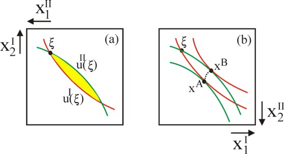
Note that the curve of II is concave in the system of axes of I, because she is rotated over an angle of 180o. Therefore the curves intersect on a second location, besides the initial point ξI = ξII. In the displayed situation the individual I prefers more of the good 1, and the individual II prefers more of the good 2. That is convenient. This is also clear from the tangents of the two indifference curves in the intial point, which have different slopes. For that slope is precisely the marginal rate of substitution. In the initial point she is larger for I than for II. The individual I has a relative preference for the substitution of goods 2 in favour of more goods 1.
Apparently there is room for exchange and redistribution. The reader will understand, that the exchange process must end at the moment, when the MRS of the two individuals has become equal. In a mathematical form this is MRSI = MRSII. In a graphical sense this end point implies, that there the tangents of the two indifference curves coincide. Such points are called Pareto-optimal. The characteristic of the Pareto-optimal situations is, that no individual can raise his utility without reducing the utility of other individuals.
This does by no means imply, that a Pareto optimal situation is just4. The injustice is illustrated in the figure 2b. Consider first the Pareto-optimal point xA. Here the individual II, starting from the indifference curve with value uII(ξII), has succeeded in continuously raising his utility by means of exchange. In the end point, where one has MRSI(A) = MRSII(A), the individual I still has his original utility uI(ξI). During the entire exchange process the individual II has been able to carry through the exchanges, which favour him most. Therefore he is called an option-setter. The passive partner in the exchange is called the option-taker5.
It is obvious, that the individual I would also like to be the option-setter. When he succeeds, then he can raise his own utility, while the utility of the individual II remains equal to uII(ξII). Then the Pareto-optimal end point is given by xB. See the figure 2b. The points xA and xB are called exploitation points, because of the imbalance in the exchange. Apparently factors of power play a role, which favour one individual.
Naturally more balanced exchange processes are conceivable. Their end points lie between the points xA and xB. Each point is again the point of contact of two indifference curves, one of I and one of II. Together the points form the so-called contract-curve, also called the core6. Without additional information it can not be predicted, where on the contract-curve the end point of the exchange process will be located. Although the points on the contract-curve are stopping places, there is no unique equilibrium! This is not the familiar market of the Walrasian equilibrium theory7.
An essential hallmark of the Walrasian equilibrium model is, that the consumers are price-takers8. They try to maximize their utility within the limits, that are imposed by the competitive market. The prices emerge from the balance of the total effective demand and the total supply. The interpersonal interactions of the barter economy are replaced by the price fluctuations, which together must guarantee the clearing of all commodity markets. A unique competitive equilibrium is formed. In the present situation, with the Edgeworth box, there are just two goods. Therefore the decisive market variable is the price ratio p2 / p1, where pn is the price of good n (n=1,2).
First consider again the situation of a single individual9. The individual possesses quantities ξ of the goods 1 and 2. Since in this situation he is a price-taker, the price-ratio is a given for him. Then he disposes of a budget y with a value of p1 × (ξ1 + ξ2 × p2/p1). The price p1 can be used as a scaling factor (also called the numéraire), so that the scaled budget is represented by y/p1.
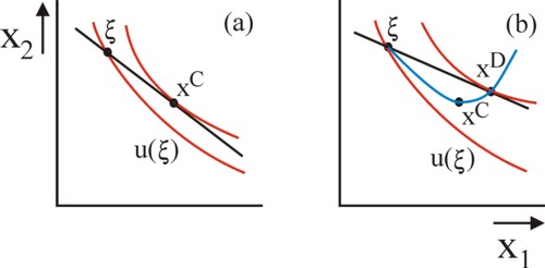
Starting from his preferences, embodied in his field of indifference curves, the individual can now search for a package of goods x with a larger utility. For that purpose he must sell goods in order to buy other goods. Since his budget is y/p1, his budget line is given by the vectors x, that satisfy y/p1 = x1 + x2 × p2/p1. The figure 3a shows this budget line in a graphical manner, together with several indifference curves from the total field of the individual.
The maximization of the utility of the individual implies, that he searches for the indifference curve with the largest value of utility, which is still located on the budget line. This is naturally the curve, which just touches the line. Designate the point of contact by the symbol xC. This point is called the consumer optimum. Apparently for the given price ration the demand of the individual equals here a quantity x1C − ξ1 of the good 1, and his offer equals a quantity ξ2 − x2C of the good 2.
The demand and the offer of the individual in the consumer optimum are clearly dependent on the price. The figure 3b shows, for the same individual but for another price ratio, the end point and the consumer optimum xD. In a similar manner for all possible price ratios the demand and the offer of the individual can be constructed. Together all these points form the so-called offer curve of the individual, in the terminology of the economist A. Marshall.
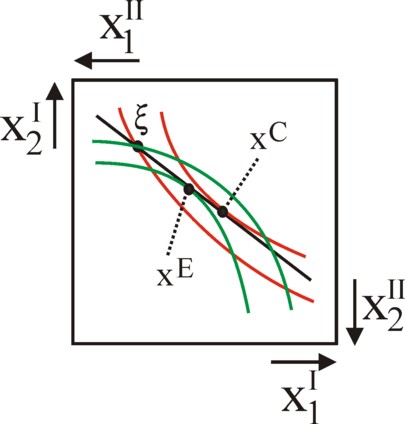
Now designate again this individual with I, and suppose that there is a second individual II. The exchange curve can also be constructed for this individual. Before discussing the general case of the fan of budget lines through ξ, first a study is presented for the price ratio p2/p1, which prompted the individual I to choose xC (see the figure 3a)10. Suppose that this price ratio incites the individual II to choose quantities xE. This situation can be displayed in the Edgeworth box, together with the budget line. She is shown in the figure 4. It is noteworthy, that the budget lines of I and II coincide11.
The reader sees in the figure 4, that the consumer optima of I and II (respectively xC and xE) are separated. This implies, that for this price ratio there is to much demand for the good 1, and not enough demand for the good 2. The market for the good 2 is not cleared. The nature of markets is such, that the price of the good 1 can rise, whereas the price of the good 2 must fall. Therefore the slope of the budget line will increase. This price change will continue, until finally the two consumer optima coincide. This unique point xC = xE for a price ratio pCE is called the top level optimum.
In the top level optimum the two indifference curves touch each other. Therefore one has MRSI = MRSII, so that it is Pareto optimal and located on the contract curve. There the MRS exactly equals the price ratio pCE. This is the requirement, which must be satisfied in the equilibrium state.
Thus it is illustrated how that equilibrium can emerge by means of a price adjustment on the market. An alternative way of argumentation uses the exchange curve (see the figure 3)12. Both the individual I and II have their own exchange curve. The two exchange curves can be drawn in the Edgeworth box. The top level optimum is located in the intersection of the two curves. By definition the budget line touches in that point both the indifference curve of I and the indifference curve of II. This ensures the Pareto optimal state.
In the preceding paragraph the Edgeworth box is used merely as an instrument in order to clarify the arguments. For on the competitive market the exchange is no longer a bilateral process, but it is multi-lateral. Each new entrant on the market makes the contract curve (or core) shrink further, until finally for an infinite amount of individuals just one shared point in the box remains13. A multitude of individuals results in a situation, where a relatively limited space is left for bartering. Here the Edgeworth box serves mainly to illustrate how the preferences of the individual still influence the market price, although in the end he has become a price-taker.
The argument of the preceding paragraphs forms the foundation of the well-known first fundamental theorem of welfare economics. This states: "When all individuals have monotonous egocentric utility functions, and when (xC, pCE) is the competitive equilibrium, then xC is located on the contract line, and thus is Pareto optimal"14. It is clear, that the reverse of the theorem does not hold.
This is illustrated for instance by the point xA in the figure 2b. Suppose that the price ratio is such, that this point is located in the budget line. Then the line has a slope, which exceeds the MRS. That is to say, the individuals I and II believe in the point xA, that p1 is too large in comparison with p2. They both want to sell the good 1, and buy more of the good 2. Apparently the market demand and the market supply are not balanced. There is no competitive equilibrium15. The point xA can only be reached due to the special position of power of individual II.
Although the Walrasian exchange model above has undeniably a formal elegance, it can not be applied to the real economy. For it is not really possible to include the economic dynamics in the model. The dynamics is present in the various variables, for instance in the budget y of the individuals. For the budgets are continuously supplemented due to the incomes. The incomes themselves are again dependent on the preferences of the individuals. Thus the wage level (the price of the factor labour) is partly determined by the number of hours, that a person is willing to work. See the column about this theme. So the consumer market turns out to be connected with the market for production factors16.
The exchange process of consumer goods can not be separated from the production. It is clear that the price changes on the commodity markets can merely be realized, as far as the production process allows for them. The product price can never fall below the cost-price. And the wage level and the interest rate, which determine the costs, are again dependent on the productivity of the production factors labour and capital. Thus the budget line of the individual can take on various forms, depending on the institutions and adjustments of the economic structure. The determining factors and conditions for the competitive Walrasian equilibrium have already been summarized, albeit succinct, in a previous column. The detailed explanation of the complete model starts with the establishment of the Edgeworth box for the allocation of the production factors labour and capital. This subject will be treated in a future column.
Evidently the market for the production factors is very time-sensitive. The expectations determine, whether the producers are willing to invest in the production capital. This kind of decisions can not be displayed by indifference curves. Moreover in such a complex system it is totally unclear, how the individuals together will ever find the Walrasian equilibrium. As soon as a price change disturbs the equilibrium, the Walrasian model can no longer be applied. The economist Sraffa has shown, that a price change has unexpected effects on all other product prices. This phenomenon has been described in a previous column.
This shows that especially the modelling of the production creates problems. For instance, the Walrasian theory of the production also supposes, that in the production no scaling effects will occur. It is obvious that this assumption is not realistic, but she is an unavoidable consequence of the assumption of a competitive market. Besides in the real economy the mediation of the money as the means of exchange turns out to be anything but neutral. She generates an abundance of side effects17.