The neoricardian theory of Piero Sraffa
First insertion on Heterodoxe Gazet Sam de Wolff: 13 june 2012
E.A. Bakkum is professionally active in the Sociaal Consultatiekantoor, where he holds the position of solicitor. He loves to reflect on the labour movement.
In 1960 the economist Piero Sraffa published the book Production of commodities by means of commodities1, that would radically change the thinking about the macro-economic development. Notably the contents implies an effective refutation of the marginalist analysis of macro-economics, which until that moment was leading. The shock among the neoclassical economists was enormous. Even now, half a century later, still many neoclassicial economists suffer from a psychological repression, and prefer to simpy ignore the work of Sraffa. Especially the North-American economists have difficulty in facing the modern insights. For instance in the popular text-book Macro economics by N. Gregory Mankiw one searches in vain for a mention of the theory of Sraffa. Since this book is used as subject-matter for tuition at the Dutch universities, whole generations of students are formed in blissful ignorance. This shortcoming is the main reason to explain in the present column once again the ideas of Sraffa2. Your columnist undertakes this with some feeling of substituting shame.
In addition to the disastrous implications for the neoclassical theory of macro-economics, the theory of Sraffa has also undermined the marxist labour theory of value. In the sixties of the last century this was an important feat of arms, because then the theory of Marx was still the state doctrine of the Leninist power block in Eastern Europe and in Asia. The marxist economists preferred the same way of acting as the present American economists, and conveniently ignored the discoveries of Sraffa.
The theory of Sraffa goes on from the works of the classical economists, notably David Ricardo, and therefore is sometimes called the neoricardian theory. For Sraffa interprets the profit as the income, that remains after the payment of the wages. With this he distances himself from the neoclassical idea, that the profit emerges from the marginal productivity of the factor capital. To be concrete, the theory of Sraffa has some important consequences:
- A wage-profit curve is derived on the macro-economic level. This provides for a clear illustration of the conflict of interests between the production factors labour and capital, which so intensely fascinated the classical economists like Adam Smith, David Ricardo and Karl Marx.
- It is shown, that the production factor capital is merely a fiction. For its calculation requires the summation of the values of the already present capital goods. And these values in turn depend on the chosen distribution of income, that is to say, the height of the wage level and the general profit rate. Therefore it is impossible to calculate the wages and the profits from the marginal products of the production factors, like the neoclassical theory attempts. To put it differently, the capital goods can not be aggregated in a meaningful way.
- The aggregation problem also undermines the marxist theory, at least its simultaneous variant. Also Marx assumes, that the total social capital is simply the sum of the values of the separate capital goods. Here he uses the labour theory of value to justify his assumption. Sraffa shows, that the labour theory of value leads to a wrong calculation of the prices, and thus of the capital3.
The theory of Sraffa makes several assumptions in advance (like any other). One can mention:
- The description is static, so that there is no room for the natural economic dynamics. The producers can only choose from the existing production techniques. The technological progress, and thus the innovation, are ignored. The growth due to the rising labour productivity is not included. Therefore the theory is not suited for descriptions of the long term4.
- There are no positive scale effects. A scaling-up does not change the proportions of production. The English expression for this neutrality is constant returns to scale. Incidentally this unrealistic assumption is found more often, for instance also in the neoclassical theory5.
- The formation of prices takes place through a markup on the production costs. The producers calculate their price by means of the universal profit rate. Moreover one produces just enough to satisfy the demand on the markets. Thus the price formation due to scarcity is not described by the theory
In this column the theory of Sraffa will be explained by means of a simple example, that is reproduced from the draft reader Vooruitgang der economische wetenschap, published in 2011 by Uitgeverij E. de Bibelude6. The example is an economic system with two branches. One is the agriculture, that is active in the production of corn (measured in bags). The other branch is the industry, and she produces metal (measured in tons, or to put it differently 1000 kg). Both branches use a part of the produced corn and metal for themselves as means of production (in the form of seeds for sowing, fuel, tools etcetera). Evidently each branch employs workers. Their wages are paid in advance in bags of corn (for bread, gin etcetera) and tons of metal (for domestic appliances etcetera). Concrete the branch for corn uses yearly qggmglg workers. He produces yearly Qg bags of corn. Likewise the means of production in the branch for metal are yearly qgm bags of corn, qmm tons of metal, and lm workers, and the production is Qm tons of metal. An analyses such as this one, which is restricted to quantities, is called an (open) Leontief-system.
The absence of growth implies that the economic system maintains itself. If another technique would be selected, then probably the values of qgg, qmg, lg, qgm, qmm, and lm would change. What remains after the subtraction of the quantities of the means of production is called the nett product of the economy. These are Qg,N and Qm,N, for respectively the agriculture and the industry. They are determined from
(1a) Qg,N = Qg − qgg − qgm
(1b) Qm,N = Qm − qmg − qmm
The wages and the profits are paid from the nett product. Table 1 shows the values, that will be used in the present example.
Table 1: core variables of the economic system consisting of agriculture and industry
Source: paragraph 6.1 in Vooruitgang der economische wetenschap
| agriculture | industry | nett product |
|---|
| corn | qgg=5 | qgm=4 | Qg,N=3 |
| metal | qmg=0.2 | qmm=2 | Qm,N=0.9 |
| workers | lg=20 | lm=10 | |
| production | Qg=12 | Qm=3.1 | |
It is practical to rewrite the formulas 1a-b as
(2a) Qg,N = Qg × (1 − agg) − Qm × agm
(2b) Qm,N = - Qg × amg + Qm × (1 − amm)
Here the a's are defined according to agm = qgm/Qm etcetera. The a's are simply the scaling factors, that describe the proportional growth of the means of production in case of a rising production. Their magnitude depends only on the production technique, and therefore they are called the production coefficients. In a similar way one defines ag = lg/Qg and am = lm/Qm, and calls them the labour coefficients. The toal is called the technical coefficients of the system. Table 2 summarizes the values of the coefficients, as they are derived from the table 1.
Table 2: technical coefficients
Source: paragraph 6.1 idem
| agriculture | industry |
|---|
| corn | agg=0.4167 | agm=1.290 |
| metal | amg=0.01667 | amm=0.6452 |
| workers | ag=1.667 | am=3.226 |
This type of tables is well suited for a planned management of the production. But in the economic market system the distribution of goods is usually executed on the market, in a process of bargaining. This kind of distribution is based on the exchange relations of the goods and the production factors. In the present two-branche model the exchange relations are determined by the price pg of a bag of corn, the price pm of a ton of metal, and the nominal wage level w of the workers. Moreover the producers want to make a profit in the sale of their products. In particular the producers are interested in the profit rate r (the capital output). The producers in the agriculture advance a sum pg×qgg + pm×qmg. To them this sum is an investment, which they want to get back, with on top the profit, that is equal to r. Also they must pay in advance the wage sum w×lg. Sraffa assumes, that the wages are not advanced, but are paid afterwards from the yield. The sale of the corn yields pg×Qg 7. In this case the price formula of Sraffa is given by
(3a) pg×Qg = (pg×qgg + pm×qmg) × (1+r) + w×lg
Completely analogous one finds for the industry the formula
(3b) pm×Qm = (pm×qgm + pm×qmm) × (1+r) + w×lm
Also here it is convenient to change to formulas, that only contain the technical coefficients. One finds
(4a) pg = (pg×agg + pm×amg) × (1+r) + w×ag
(4b) pm = (pg×agm + pm×amm) × (1+r) + w×am
Note that in each equation of the system the indices of the coefficients are interchanged with respect to those in the system 2. The two equations 4a-b contain 3 unknowns, namely pg, pm, and w. The solution of this system requires a third equation. Sraffa proposes as a third equation to use one of the products as the unit good. Then this unit good plays henceforth the role of money, which can express the prices of the other goods. Take for instance pg=1. Then one finds the values pm and w, expressed in bags of corn. In fact the assumption pg=1 implies simply a division by pg of the left and right sides of the formulas 4a-b. To put it differently, actually pm/pg and w/pg are solved from the formulas 4a-b. The quantity pg is used here as the so-called numéraire of the system.
The system 4a-b can be solved by a substitution of variables. In somewhat larger systems this soon becomes a complex matter. In those cases the matrix calculation is a convenient instrument. Therefore your columnist chooses also in the present case the matrix notation8. Then the system of equations 4a-b gets the form
(5) p = (p · A) × (1+r) + w×a
In the formula 5 p is the horizontal vector [pg, pm] voor, a is the horizontal vector [ag, am], and A is the 2×2 matrix with rows (from the top downward) [agg, agm] and [amg, amm]. The solution of the formula 5 is
(6) p = a · (I - A×(1+r))-1 × w

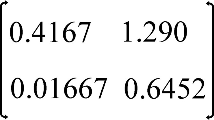
Figure 1: Matrix A
(see table 2)
In the formula 6 I is the unity matrix, and the upper index -1 indicates that the inverse matrix of I - A×(1+r) should be employed. In case of the coefficients from the table 2 the matrix A has the form of the figure 1. From this the inverse matrix (I - A×(1+r))-1 is calculated with as rows
[0.3548 − 0.6542×r, 1.290 × (1+r)]/Δ and
[0.01667 × (1+r), 0.5833 − 0.4167×r]/Δ,
where Δ = 0.2474 × (r-1.146)2 − 0.1396.
Here Δ is the determinant of I - A×(1+r). The determinant turns out to be positive from r=0 until r=0.395. The vector formula 6 can again be transformed into a set of equations:
(7a) pg × Δ = (0.6425 − 1.022×r) × w
(7b) pm × Δ = (4.032 + 0.8062×r) × w

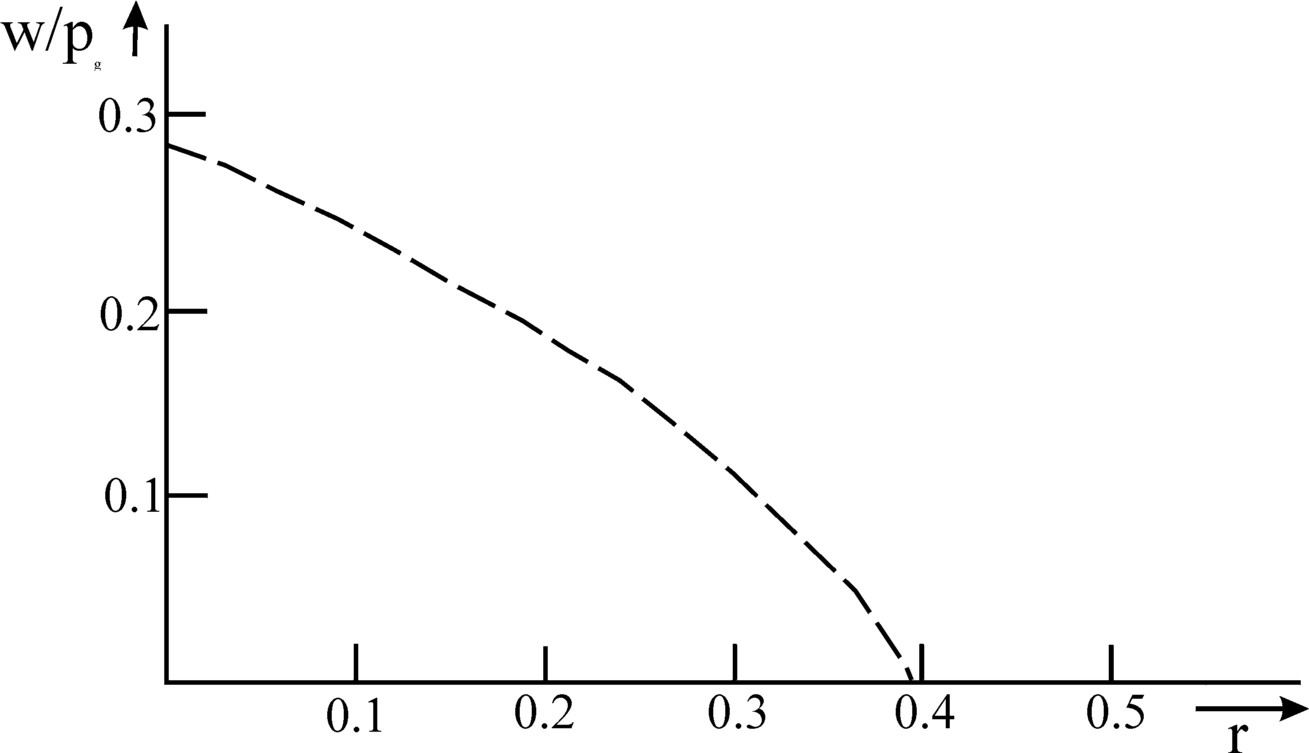
Figure 2: Wage curve w/pg belonging to the formula 8
The formulas 7a-b contain all relevant information about the behaviour of the economic system. For instance one finds from the formula 7a that
(8) w/pg = Δ / (0.6425 − 1.022×r)
This is precisely the wage curve of the system. She shows how the nominal wage (expressed in the price of a unit of corn) varies as a function of the profitability r. In the point r=0.395 the wage level has fallen to zero, so that the whole nett product goes into the profit. If on the other hand the workers succeed in claiming the whole nett product, then the profit rate will be equal to zero. Then the wage is w=0.287×pg. Tt can simply be verified, that w/pg falls continuously for a rising r. This proves the conflict of interests between the workers and the producers (or the capital owners). It can also be derived from the formula 8, that the fall in the wage level accelerates, according as r increases. In other words, the second derivative of w/pg with respect to r is (also) negative. The course of the wage curve is show graphically in the figure 2. One sees how the curve as it were turns away its convex side from the coordinate axes. Such a course of a curve is called concave.
The theory of Sraffa has the interesting property, that she shows how the product prices change, when the distribution of the nett product between the workers (wage) and the producers (profit) is modified. In the used example the formulas 7a-b show clearly, that the ratio pm/pgm/pg=6.251. And for r=rmax=0.395 the price ratio has become 18.03 9. Apparently in the case of a rising profit rate r the metal becomes relatively expensive with respect to the corn. This illustrates also the relative meaning of the nominal wage w, because it is not decisive for the real purchasing power. For a rising price of metal implies, that the workers can actually buy less metal with their wage w.
Another important economic quantity is the so-called capital intensity κ, that is to say the costs of the used means of production per hired worker10. The total costs of the means of production in the whole economy consist of the sum of the costs in the separate branches, so of (pg×qgg + pm×qmg) + (pg×qgm + pm×qmm). The total number of hired workers is lg + lm. Of course κ, which is also simply a price sum, must be normalized with the numéraire pg. The result is
(9) κ/pg = ((qgg + pm×qmg/pg) + (qgm + pm×qmm/pg)) / (lg+lm) =
((agg + pm×amg/pg) × lg/ag + (agm + pm×amm/pg) × lm/am) / (lg+lm) =
((agg + amg×(pm/pg)) × lg/ag + (agm + amm×(pm/pg)) × lm/am) / (lg+lm)
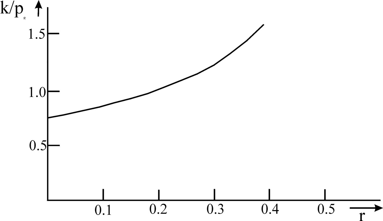
In the preceding parapgraph is it established, that the size of the ratio pm/pg depends only on the profitability r. According to the formula 9 this also holds for the capital intensity κ/pg, at least as long as the production technique is given and thus the technical coefficients are fixed. Your columnist forgoes the task to rewrite the formula 9 as a function of r. But the figure 3 does show, how κ/pg varies with r.

Figure 3: Capital-intensity κ/pg as a function of the profit rate r
(calculated with formula 9)
The figure 3 shows a surprising relation between the capital intensity and the profitability r. For it appears, that the capital intensity rises, when the profitability increases. This implies, that the producer invests more in capital goods for each worker, according as that same capital should yield a larger profitability. In a world with perfect competition one would expect just the opposite. For in that case the profit of enterprises on the macro-economic level is zero. Then the profitability is the price, which the producer must pay for the employment of the capital goods. One would expect, that in the case of a rising price of capital the producer would diminish his investments in capital goods per worker. For it becomes more attractive to substitute the factor labour in place of the factor capital. Such a behaviour is indeed precisely the functional coherence, that is expected on the basis of the neoclassical theory. In the neoclassical theory the expensive production factors are replaced by cheaper ones. Figure 3, and thus the theory of Sraffa, proves that the idea of the neoclassical theory is too superficial and wrong. With this the whole macro-economic interpretation of the neoclassical theory is refuted.
Incidentally the theory of Sraffa shows, that the course of the capital intensity κ/pg as a function of r is dependent on the production technique, that the producers have chosen. There are also techniques, where the behaviour as predicted by the neoclassical theory does occur, and thus the capital intensity decreases for a rising profitability. Characteristic for this kind of techniques is, that the wage curve w/pg has a convex shape, or to put it differently, her convex side is turned towards the coordinate axes11. When the producers choose the productions techniques, it is not the relation between κ/pg and r that matters, but the realization of the maximal profit rate at a given wage level12.
Finally it should be remarked again, that in the example just presented the change of the capital intensity is not caused by physical modifications. For at the start it has been stated, that the material system simply maintains itself (reproduction). The quantities qgg, qgm, qmg, and qmm do not change. The only thing that changes, is their value, at least as long as the distribution of the nett product varies. And for the producers only the value counts (and not the physical quantities), because the profitability is calculated on the basis of the value of capital. If more capital is invested (taken as a price sum), then they are obliged to produce more profit.
- See Production of commodities by means of commodities, (1960, Cambridge University Press). (back)
- Your columnist owes his knowledge to two books, namely Grundzüge der neoricardianischen Preis- und Verteilungstheorie (2000, Metropolis Verlag) by E. Feess-Dörr, and Lectures on the theory of production (1977, Macmillan) by L.L. Pasinetti. Both books excel by their clarity and completeness. But of course many other good books about the theme have been published. (back)
- Here Sraffa assumes that the prices remain unchanged. In the bookkeeping of the producers the prices of purchases and sales are identical, as if they are determined simultaneously. In the model the changes of prices are not considered. It is the merit of the economist Andrew Kliman to call attention to this special aspect of the approach of Sraffa. (back)
- The marxist economist A. Müller (incidentally from West Germany) states that these assumptions of Sraffa are unrealistic. In a static situation the economic signals are lacking, which may motivate the producers to invest. At the time this argument was also used by the Leninist economists from the Soviet imperium. But none of them can explain, how this urge to innovate should be modelled in a theory. (back)
- Also this point was seized by the marxist economists, in order to discredit the theory of Sraffa. For in the theory of Marx the producers are forced to keep accumulating, because they for ever want to outdo their competitors in efficiency. Thanks to the accumulation they work up the labour productivity. (back)
- See chapter 6 of Vooruitgang der economische wetenschap (2011, E. de Bibelude), by E.A. Bakkum. Uitgeverij E. de Bibelude is a part of the Sociaal Consultatiekantoor. (back)
- It has already been remarked, that here the simultaneous character of the theory of Sraffa becomes visible. (back)
- Readers who are unfamiliar with the matrix notation can solve the formulas 4a-b by themselves by means of substitution. But if they are fascinated by the matter, then perhaps it is worth while to buy a text book about linear algebra, and to appropriate the matrix calculations. Also the system 2 becomes simpler in matrix notation, namely QN = (I − A) · Q. Here I is the unity matrix. Note that here the vector Q appears on the righthand side of the matrix A. The transposed (with symbol †) of the quantities equation should be taken in order to get the same form as the price equation: Q†N = Q† · (I − A†). This transforms the vertical (column) vectors into horizontal (row) vectors. The similarity of the systems of quantities and prices is called duality. (back)
- The ratio pm/pg can be found by dividing the formula 7a by the formula 7b. Then on the right hand side of the equation the wage w drops out, so that the resulting expression depends only on r. (back).
- In fact the calculation of the capital intensity should distinguish between on the one hand the circulating means of production, such as raw materials, and on the other hand the fixed capital goods, such as machinery. Then the capital intensity refers only to the fixed capital. For the sake of simplicity here the difference is ignored. (back)
- The system in table 3 turns out to be such a production technique. See for the elaboration of the example in the table 3 the paragraph 6.5 in Vooruitgang der economische wetenschap. (back)
- In principle the producers always try to make their profit maximal, certainly in a system of competing enterprises. The theory of Sraffa does not interpret the profit rate r (that is to say, the profitability) in an unambigeous way. It is simply the markup of the production costs, which must pay for the profit of the entrepreneur, and certain production costs like the interest of capital, the rent of land, and taxes. In the neoclassical theory with perfect competition the aggregate profit of the entrepreneurs is zero. Then in many text-books it is assumed, that the profitability accrues completely to the capital owners, so that r would be identical to the interest rate. (back)
Table 3: core values of an economic system consisting of agriculture and industry
Source: paragraph 6.5 in Vooruitgang der economische wetenschap
| agriculture | industry | nett product |
|---|
| corn | qgg=11.5 | qgm=2.573 | Qg,N=7.927 |
| metal | qmg=1 | qmm=0.0393 | Qm,N=0.1987 |
| workers | lg=20 | lm=10 | |
| production | Qg=22 | Qm=1.238 | |
