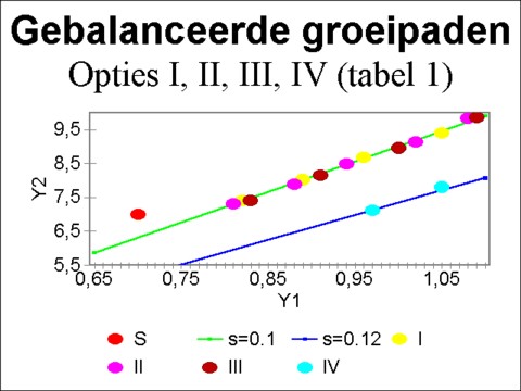
Figure 1: Balanced growth paths
of table 1. Initial point Y = (0.7, 7)
After the discussions of various types of one-sector models in the previous columns, the present column studies two-sector models. They originate again from the book Mathematical models of economic growth1 by Jan Tinbergen. These models allow to study the economic structure, just like the theory of Sraffa. Thus the path of balanced growth can be found. Moreover, the utilization of the production capacity can be optimized during the indispensable previous period of adaptation. This type of theories with an investment function are indeed dynamic. The two-sector models form the link between the macro-economics and the structure models2 in micro-economics.
The two-sector models build on the production schemes of Karl Marx. However, they ignore the distribution of the product, contrary to Marx, who distinguishes between the incomes from wages and profit. The models have a peculiarity, which must be metioned to the reader as a warning. Namely, all variables are aggregated, so that their size expresses the monetary value, and not the physical quantities. This causes problems, as soon as the production technology changes, for instance when another capital coefficient is preferred. For, then the production prices must change, and thus the monetary values. Tinbergen assumes that the prices remain constant, but for the case of technical innovation that is evidently strange.
In this paragraph a growth model with two sectors is described, namely the production of investment- and consumption-goods3. In fact the model will be presented with an arbitrary large number of consumption sectors, instead of merely one. The extension to several consumption sectors is naturally convenient for the practice of planning, but it does not add any insight. Investments lead to economic growth, so that the model is dynamic. In principe all variables are a function of the time t.
The sector for the production of investment- or capital-goods gets the index n=1. This sector must produce all equipment for the economic system. Therefore the size of the sector-product (or the earned income there, which in the given circumstances amounts to the same) is Y1(t) = I(t), where I(t) is the investment volume at the time t. It is assumed, that the investments are exactly covered by the savings, so that one has I(t) = S(t). As usual, the sum of the savings is represented by the formula S(t) = σ × Y(t), where σ is the savings rate and Y(t) is the social product, that is to say, the national income.
The national income is composed of the separate incomes Yn of all n sectors. It is calculated from
(1) Y(t) = Σn=1N Yn(t)
In the sectors n=2, ..., N the consumption- or end-goods are produced. Each sector disposes of a quantity Kn(t) of capital goods or equipment. The investment in the sector n satisfies In(t) = ∂Kn/∂t = ∂(κn × Yn(t)) / ∂t = κn × ∂Yn/∂t, where κn is the capital coefficient of the concerned sector. It is assumed that κn does not depend on time.
Besides, there is a lag θ before activating the investment. For, the producers will generally not be able to deliver immediately after the placement of the order. The investment is spread in a uniform manner over the period θ, which is needed in order to produce the equipment and install it. Due to the lag θ the income Yn(t) is not directly affected by the investment. Suppose for the sake of convenience, that the lag is identical for all sectors. Then the investment function has the form
(2) In(t) = κn × (Yn(t + θ) − Yn(t)) / θ
In accordance with the formule 1 one has I(t) = Σn=1N In(t). Since the product of the sectors with n>1 is consumed, one has for these sectors that Yn = Cn(t). For, on an equilibrated market the supply and demand are equal. The total consumption C(t) is the difference of the income and the savings. In formula this is C(t) = Y(t) − S(t) = (1-σ) × Y(t). Suppose that the consumptive demand for the product of the sector n contains an autonomous component Γn, and an income-dependent component γn × C(t). Then the consumption function for the product n has the form
(3) Cn(t) = γn × (1 − σ) × Y(t) + Γn
The constants gamma;n are called the marginal propensities to consume of the products n. Due to the distinction between the investment- and consumption-goods the sector 1 does not have its own consumption function. Furthermore, note that the assumption C = Y-I implies, that consumptive expenses are never covered with credits. Then the formula 3 implies that C × Σn=2N (1 − γn) = Σn=2N Γn. Suppose that both sides of the equation have the value zero, than one has Σn=2N γn = 1.
In general the described model will be used only in the second phase of the planning procedure. In the first phase a simple one-sector model will be used to determine the savings rate σ, because she is essential for the desired growth rate of the economy as a whole. As soon as a certain value of σ has been selected, then the most desirable structure can be chosen next, for instance by means of the presented model. The structure must be fairly durable, because otherwise the markets will destabilize. Such a planning process can be performed as an iteration, so that after the second phase of the planning process the policy makers return to the first phase, in order to adjust the value of σ.
The model in this paragraph is solved by combining the formula 1 with the identities for the market equilibria S=I and Yn=Cn (with n>1). In this way the formulas 2 en 3 can be expressed completely in terms of Yn. One finds:
(4a) σ × Σm=1N Ym(t) = Σm=1N κm × (Ym(t + θ) − Ym(t)) / θ
(4b) Yn(t) = Γn + γn × (1 − σ) × Σm=1N Ym(t) (n>1)
The system 4a-b can be brought in the shape of a matrix equation. Namely, she is equal to
(5a) Σm=1N κm × Ym(t) = Σm=1N (κm + σ×θ) × Ym(t − θ)
(5b) Σm=1N (δnm − γn × (1 − σ)) × Ym(t) = Γn (n>1)
In the formula 5b δnm is the well-known mathematical Kronecker delta;. The system 5a-b has the form A · Y(t) = b, where A represents a n×n matrix, Y(t) is a 1×n vector with as its elements Yn(t), and b is a constant vector.
That is to say, the elements of the matrix A are a1m = κm, and for n>1 anm = δnm − γn × (1 − σ). The vector b has the elements b1 = Σm=1N (κm + σ×θ) × Ym(t − θ), and for n>1 bn = Γn. It is true that b1 depends on t-θ, but yet this is not a constant value, since at the time t the quantities at the time t-θ are already completely known.
Thus the model is brought in a form, which allows for a simple solution. For, now one has Y(t) = A-1 · b, where A-1 is the inverse matrix of A. Here it is striking, that not all Yn(t-θ) must necessarily be known, but merely the quantity b1. Apparently b1 determines the growth rate g of the system. Suppose that a solution is searched with a uniform growth rate for all sectors. This is called the balanced growth, because the time does not change the structure of the sectors. In order to calculate the growth rate from b1, it is convenient to try the solution Y(t) = η ×eg×t + ζ. She can be inserted into the formula 5a, so in Σm=1N a1m × Ym(t) = b1(t-θ). The result is4
(6) Σm=1N (κm × (eg×θ − 1) - σ×θ) × ηm = 0
The same solution can be tried in the formula 5b, so in Σm=1N anm × Ym(t) = Γn with n>1. Since the right-hand side does not depend on time, one must have Σm=1N anm × ηm = 0. Define a new matrix A'(g) with elements a'1m = κm × (eg×θ − 1) - σ×θ and for n>1 a'nm = anm. Then the matrix A'(g) apparently has the eigenvector η with eigenvalue zero. That is only possible when the determinant of A'(g) equals zero. This determinant equation allows to calculate the value of g.
Now that the right growth rate g has been found, which is reconcilable with b1, η can be calculated from A' · η = 0. In the same way the insertion into 5a-b yields a set of equations for ζ, which allows to solve ζ 5. Note that η is an eigenvector of A', and therefore is known, apart from a scaling factor. However, this scaling factor can be calculated from the initial condition Y(t-θ) = η × eg × (t-θ) + ζ. This completes the solution of the problem. Tinbergen calls this case exceptional. For, apparently in an arbitrary initial state Y(t-θ) a path of balanced growth can be reached in a single time step θ, so that henceforth all sectors have the growth rate g.
In fact this model is simply a method of bookkeeping of the quantity of capital goods. The initial capital is expanded by means of the newly invested capital. The policy maker (for instance, the planning agency) must redistribute the capital in the initial situation over all sectors in such a manner, that henceforth the balanced growth will be guaranteed. The redistribution also fixes the structure. The path of balanced growth is reached in the period θ of adaptation. Note, that the development Y(t) = η ×eg×t + ζ begins after the adaptation, but does not hold during the process of adaptation.
It is a merit of this model, that an arbitrary number of sectors for consumer goods is modelled. But the reader may notice, that, except for the sector 1, no interaction between the sectors is present. In this respect the model is more primitive than for instance the three-sector models of Biersack (with an extra sector for the production of raw materials) and of Feldman (with an extra sector for the production of equipment for the production of machinery, the so-called second order capital goods).
The presented model can be illustrated well by means of an example, which besides the sector 1 has an additional sector for the production of consumer goods. Then one has by definition γ2=1 and Γ2=0. Moreover, the formula 5b shows that one must have η2 = (1/σ − 1) × η1. Due to Γ2=0, this simple example leads to ζ=0. Apparently the desired growth path in the (Y1, Y2)-plane is the line through the origin with slope (1/σ) − 1. The requirement, that the matrix A'(g) must have a determinant with a value of zero, fixes the growth rate for the balanced development
(7) g = ln(1 + θ / (κ1 − κ2 + κ2/σ)) / θ
Suppose that the initial state of the system is determined by Y1(0) = 0.7 and Y2(0) = 7. This is the red dot in the figure 1. In principle the policy maker has the free choice of σ, κ, and θ. Due to the existing stock of capital goods the choice of κ and θ is not completely free, but thanks to the investments some adaptation is possible. The table 1 sums up the values of these variables, the options, which the policy maker wants to consider. Due to the two values σ=0.1 and 0.12 there are two growth paths. In the figure they are drawn in respectively the colours light green and dark blue.
| option | σ | κ1 | κ2 | θ | g | Y1(θ) | Y2(θ) |
|---|---|---|---|---|---|---|---|
| I | 0.1 | 3 | 1 | 1 | 0.0800 | 0.823 | 7.402 |
| II | 0.1 | 4 | 1 | 1 | 0.0741 | 0.813 | 7.318 |
| III | 0.1 | 3 | 1 | 1.2 | 0.0794 | 0.823 | 7.402 |
| IV | 0.12 | 3 | 1 | 1 | 0.0924 | 0.970 | 7.114 |
For each option the growth rate is computed from the formula 7, and this is also included in the table 1. After the period θ the growth path is reached. The conservation of capital requires that the point of arrival satisfies the formula 6. Together with η2 = (1/σ − 1) × η1 that point determines the vector η. Next it can be used to compute the vector Y(θ), which indicates the point of arrival on the growth path. This vector is also included in the table 1, and besides it is drawn in the figure 1 (see for the concerned colours the legends of the figure). From the point of arrival onwards the vector will grow with a factor eg×θ for each following time step θ. The succession of points is also shown in the figure 1.
The table shows, that policy choices are rarely trivial. A high savings rate is favourable for the future (option IV: σ = 0.12), but for that option the people must temporarily diminish their consumption. The growth in the sector 1 is impetuous to such an extent, that the third point Y(3 × θ) is already located outside the figure. On the other hand, a large capital coefficient (option II) equals a low capital productivity. And a large lag in the investments (option III) turns out to slow down the growth rate. Note, that in the figure 1 for the case θ=1.2 the points Y(n × θ) have a larger intermediate time step than for θ=1. Therefore in the figure 1 the reader must not be misled by the apparently fast growth of this option III.
Most of the models, which are presented in the columns on this portal, assume that the utilization of the available capital goods is 100%. The exceptions are the column about the theory of Domar, and the column about multi-period optimization with an intertwined balance. The present paragraph will elaborate on the approach of Domar for an economic system with two sectors, namely the production of capital goods (sector 1) and the production of consumer goods (sector 2)6.
In the theory of Domar the utilization is defined as the fraction u = Y / (K/κ). From u<1 it follows directly that K > κ×Y. In the present model with two sectors there are two utilizations un (n=1, 2), and the capital coefficients κn can also differ. Now the formula 2 is no longer valid, and changes into the investment function
(8) I(t) = Σn=12 (Kn(t+1) − Kn(t))
For the sake of convenience the investment lag is ignored in the formula 8, by inserting θ=1. The consumption function is straightforward, namely C = Y − S = (1-σ) × Y. Due to C = Y2 and Y = Y1+Y2 the products of the sectors satisfy the relation Y2/Y1 = (1-σ) / σ. This relation can be written in terms of the ratio of the utilizations
(9) u2 / u1 = ((1 − σ) / σ) × (K1 / K2) × (κ2 / κ1)
The formula 9 clearly shows, that for given stocks of capital goods Kn(0) at t=0 there is only one savings rate, which allows for a complete utilization of the production capacity. When the savings rate deviates from this value, then either u1(0) or u2(0) will be less than 1. In other words, in the situation with u1(0) = u2(0) = 1 a capacity problem will occur, as soon as σ will change7.
It may seem that the problem of the variable savings rate can be solved simply by exchanging capital between the sectors, and thus bring the ratio K1/K2 in accordance with the new σ. Indeed there may be situations, where this approach will work. Incidentally, some theories are based on this assumption, especially the one-sector models, such as with scarce capital and with factor substitution.
The assumption is certainly justified, as long as the economic system continues to grow. For, then the ratio between the Kn can change by temporarily choosing a different growth rate for each sector8. The structure gradually adapts to the new σ. Then the exchange of capital between sectors is not even necessary. As long as the planning process aims at economic growth, a change of σ apparently makes the plan more complicated but not impossible.
However, Tinbergen stresses, that in situations with a weak growth or even with contraction the differentiated growth does not offer a satisfactory solution9. In that case the policy makers should try to redistribute the capital goods over the sectors10. This would imply, that for instance the capital goods for the production of consumer goods are exchangeable for the capital goods for the production of investment goods. The first category is called the first-order capital goods, and the second category is called the second-order capital goods (the loyal reader remembers the three-sector model of Feldman). In principle this chain of capital goods, which produce different capital goods, can be differentiated to an arbitrary high order.
It is clear that this exchange of capital goods between sectors is often impossible, because the machinery is constructed especially for a single production process. This will cause an acute crisis in situations, where one or more sectors actually ought to shrink in size. Then there are two possibilities. First, in the concerned sectors the utilization of the capital goods can be diminished, in the manner that is explained in the preceding paragraph. Second, in the concerned sectors the production can be maintained at the old level, at least for the time being, and the capacity can be decreased gradually by means of scrapping.
Now, as an example of the possibilities, calculations will be performed for an economy with two sectors, such as is modelled in the paragraph about the utilization. Suppose that at t=0 the policy makers want to increase the savings rate to α×σ, with α>1. At that moment the stocks of capital goods are K1(0) and K2(0). During the process of adaptation the policy makers want to keep using the available production capacity. According to the formula 9, after an adaptation period with a duration of θ the capital ratio must have been changed into
(10) K1(θ) / K2(θ) = (α×σ / (1 − α×σ)) × (κ1 / κ2)
Now suppose that no exchange of capital goods is possible. Then one must have K2(t) = K2(0) during the whole period θ. So K1 must grow with respect to the initial situation. Express the formula 8 in more general terms as I(t) = ∂K1/∂t + ∂K2/∂t. Now the policy makers will choose ∂K2/∂t=0, and thus I(t) = ∂K1/∂t. Insert I(t) = Y1(t) en K1(t) = κ1 × Y1(t), then this yields the differential equation Y1(t) = κ1 × ∂Y1/∂t. She has the solution
(11) Y1(t) = Y1(0) × et / κ1
The formula 11 shows clearly how the process of adaptation of K1 proceeds. For, due to K1 = κ1 × Y1 it is clear that K1(t) grows with the same power of e as Y1(t). As soon as the stock of capital goods will become equal to K1(θ) = K1(0) × eθ / κ1, also K1(t) will have to grow again, so that henceforth it will satisfy the formula 10. The policy makers have apparently the task to determine the duration θ of the period of adaptation, in which is used to invest exclusively in the sector 1. The duration of the period turns out to be11
(12) θ = κ1 × ln(α × (1 − σ) / (1 − α×σ))
Here it is also interesting to study the behaviour of σ(t) during the process of adaptation. For, σ(t) = S/Y = I/Y = Y1(t) / (Y1(t) + Y2(t)). Insert again the formulas Y1(t) and Y2(t) = Y2(0). Use Kn(0) / κn = Yn(0), then one has
(13) σ(t) = 1 / (1 + e-t/κ1 × (K2(0) / K1(0)) × (κ1 / κ2))
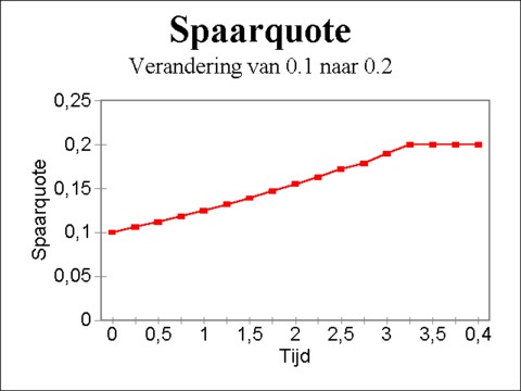
On p.61 of Mathematical models of economic growth an example is given with κ1=4, κ2/κ1 = ½, K2(0) / K1(0) = 4½, σ=0.1, and α=2. Then, according to the formula 12 one has θ = 3.24. Contrary to the model, which has been presented first, the adaptation does not take one time step, but several The figure 2 shows how the doubling of σ proceeds.