Figure 1: Boundaries in the LP problem for period 1
(single technique)
In a previous column the optimization for central planning has been described. She employs the method of linear programming. In the book Volkswirtschaftsplanung1, again a gem bought at the second-hand bookshop Helle Panke2, Hans Knop shows how some improvements can make that model applicable to reality.
The approach that has been presented in the previous column is rather schematic, and ignores important economic phenomena. This is justified for didactic reasons, because in this way the essence of the model is clarified well. In the text of Knop it is explained how the formalism can be extended in a straightforward manner in order to perform realistic calculations. Here five aspects are treated, namely (1) the distribution of the end product, (2) the choice of the production technique, (3) the foreign trade, (4) idle capacity, and (5) the delay in the installation of the investment goods.
Of course the dynamic intertwined balance remains at the core of the optimization. In a previous column the fundamental equation of the balance has been defined. She is in matrix notation
(1) ψ(t) = (I - A(t)) · x(t)
In the formula 1 t is the time variable, x is the vector of total produced quantities (in the German language the volkswirtschaftliches Gesamtprodukt), A is the intertwined matrix of the production, I is the unity matrix, and ψ is the vector of quantities of the end product (in the German terminology of Knop the Endprodukt). The formula simply expresses that the end product is the remainder of the total product, after the subtraction of the goods, that have been expended during the production. In the column about optimization it has been shown, that the boundaries on the available quantities of the various resources (labour, land, raw materials, valuta etcetera) considerably limit the possible values of x.
Optimalization requires the choice of the target function Z(t). In general she has the form
(2) Z(t) = z†(t) · x(t)
In the formula 2 z includes the weighing factors of all i products. The symbol † represents the transposition, so that z is a horizontal vector, and the formula 2 represents a mathematical inner product. A logical choice for the weighing factors z is simply the price vector p. In that case Z(t) represents the value of the total product of the national economy. For a multi-period optimization the target function must be composed of the target functions Z(t), Z(t+1), Z(t+2), .... of the separate periods. The yields of the production in the separate periods are mutually coupled by means of the investment policy.
On its own the formula 1 is unsuited for an optimization. For she suggests, that the end product ψ(t) can be made arbitrary large by chosing a sufficiently large total product x(t) of the national economy. In reality the size of x(t) is naturally bounded by the fundamental fund Γ(t-1) that is available at the start, by the size of the working population (and thus by the available labour time) B0(t), and by all sorts of non-producible resources ε (land, raw materials etcetera) with a size Rε(t).
The only extendable limitation is the stock of the fundamental fund, in a gradual manner, namely by means of the nett investments i(t). The other resources are more or less fixed, at least when a purposive increase in population is forgone, as well as the reclamation of fallows. The nett investments consist of capital goods, which must be taken from the end product. Besides also other social needs must be satisfied from the end product. Knop gives the following summary of applications3.
In summary: the national income can be written as
(6) N(t) = G · Δx(t) + Κ(t) + Δu(t)
And thus the formula 1 can be rewritten as
(7) K(t) = (I - A(t)) · x(t) − V · G · x(t-1) − G · Δx(t) − Δu(t)
Or, if desired
(8) K(t) = (I - A(t) - G) · x(t) + (I − V) · G · x(t-1) − Δu(t)
The central planning agency will in his calculations want to maximize the consumption Κ(t). Many columns on this web portal give examples of this approach. Evidently this is not equal to the maximization of the target function Z(t) in the formula 2. That target function maximizes the total product x, the end product ψ and thus also the national income N. If the planning agency fixes the rate of growth of Κ(t), then according to the formula 6 the maximization of N(t) is similar to the maximization of the nett investments i(t). This guarantees an optimal growth of the economy as a whole. And the more the economy grows, the more potential is available for eventually raising the consumption. Thus the maximization of x is in the end still equal to the maximization of Κ(t) 4.
Even a small and primitive economic system produces many thousands of products. Therefore it is in practice impossible to model the whole system in a single large intertwined balance. The central planning agency must aggregate (combine and add up) the products of the balance at the level of industrial groups or even of industrial branches (industrial sectors). If desired at the decentral or group level the intertwined balance can be refined and worked out further. Such calculations help the enterprise in making the right choices for the establishment of the production process.
Nevertheless it is sometimes even at the highest level of central planning necessary to make a choice of the production technique for a certain aggregated group. This aspect is ignored in the models, which are presented by Eva Müller5. In all the preceding columns the model assumes that prior to the optimization a choice of the production technique has been made. For each product only a single production technique has been considered.
Unfortunately it is seldom that the most desirable technique is known in advance. Actually the calculation herself should make this decision6. The production techniques can differ, because different equipment is used in the production of the same good. This occurs for the case that the production is located in different regions. It is also conceivable, that in a single enterprise old and new equipment is used at the same time. A special case occurs, when the production benefits from scale effects. That is to say, as soon as the demand for a good passes a certain threshold, a more efficient and cheaper (per unit) production process can be installed.
Here the choice for a certain production process will be illustrated by means of an example. The starting point is the formula 7, where for the sake of convenience the discarded equipment and the production-circulation fund are ignored. In other words, V=0 and Δu(t)=0. Evidently the growth requires that the circulation fund must continuously be extended. In the present simplification the investments are taken from hypothetical stocks, which have been formed in previous periods7. The production technique (matrices A and G) are assumed to be independent of time. The numerical data of the example have been copied from the earlier column about the multi-period optimization. The reader will remember, that there two branches are distinguished, namely the agriculture (corn) and the industry (metal). The boundaries on the production are determined by the initial conditions Γ(0) = [11.6, 12.7] and Κ(t) = [1.0, 0.3] × 1.1t, just like in the earlier column. Note again that here apparently not the consumption herself is maximized. For simplicity here the boundaries b(t) due to the resources are ignored.
In this paragraph the target function is defined by Zd(t) = xg + 7×xm. This definition differs from the one in the earlier column. The production of tons of metal is valued higher than the production of bales of corn. This target function is preferred here, because a previous column about the theory of Sraffa shows that the introduction of a price system will lead to a price ratio pm / pg close to 7. This fact is now expressed in the target function, which thus becomes more realistic. The target function is related to the monetary yield of the production. Incidentally this is of little importance for the present example, but it does illustrate the meaning and the use of the target function.
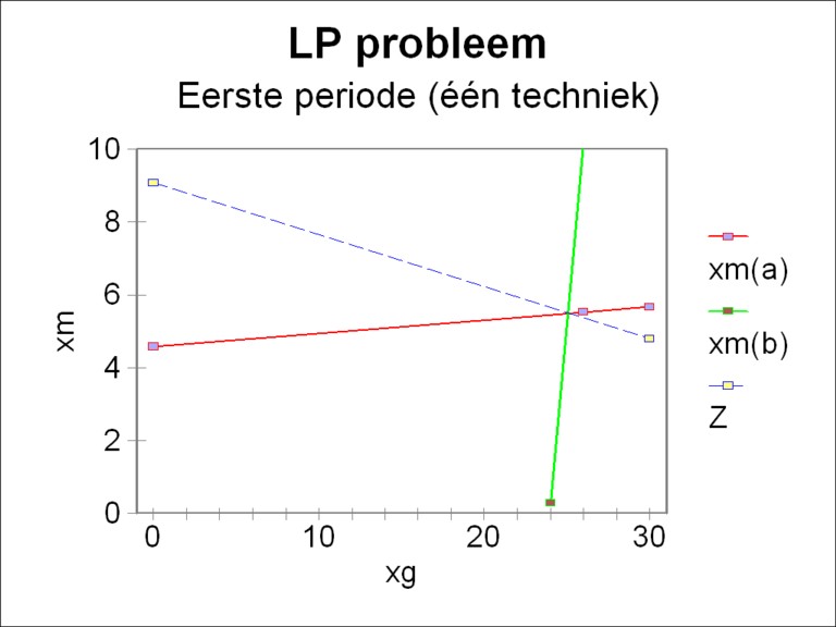
In this manner all information has been obtained that is needed for the search for the most desirable growth path. In the example a single period will be considered first, namely the time interval t=1. If this problem is solved with the method of linear programming (LP), then the optimum is found in [xg, xm] = [25.1, 5.50]. That point can be found in a graphic way, or by a calculation with the simplex method. The figure 1 is the graphic presentation.
In the present example the change will now be analyzed for the case, that the metal industry gets at her disposal a second production technique. The already existing production process (from now on indicated by 1) is characterized by the production coefficients agm1 = 1.29 (bales of corn per ton of metal), amm1 = 0.6452 (tons of metal per ton of metal), ggm1 = 1.0 and gmm1 = 0.25. The new production technique, indicated by 2, is characterized by the production coefficients agm2 = 0.9675, amm2 = 0.3226, ggm2 = 1.0 en gmm2 = 0.25. That is to say, the new technique requires the same input from the fundamental fund, but it uses 25% less corn and 50% less metal in the circulating material. Moreover it is assumed that the technique 2 can be used in an efficient way only for the case that more than 6 tons of metal are produced. Below a production of 6 tons of metal the technique 2 is not viable.
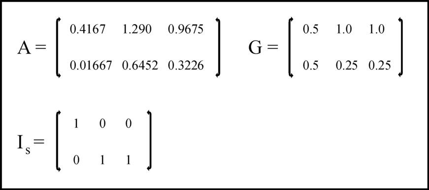
The figure 2 shows the forms of the matrices A and G for the economy with two techniques in the metal production. Besides the "unity" matrix Is is shown, which is needed in the formula 7. The matrices are no longer a square, but rectangular. The corresponding LP problem has for the first period (t=1) the following form8:
(9a) -0.0833×xg + 2.29×xm1 + 1.968×xm2 ≤ 10.5
(9b) 0.5167×xg − 0.1048×xm1 − 0.4274×xm2 ≤ 12.37
(9c) xm2 ≥ 6
(9d) xg + 7 × (xm1 + xm2) → max
The LP problem now has three variables (xg, xm1, and xm2), and can not be solved in a graphic manner. The simplex method must be used9.
The simplex method yields as the optimal point for this LP problem [xg, xm1, xm2] = [29.00, 0.4838, 6.281]. The solution is found after four simplex tableaux, in other words, after the passage of four angular points in the (xg, xm1, xm2) space. First of all it is striking that due to the introduction of the second technique the production rises both for metal and corn. The critical boundary (formula 9c) for the technique 2 is exceeded, since xm2 = 6.281. The relatively large efficiency of the technique 2 in comparison with the technique 1 makes her application attractive for the metal industry, at least for this target function. Nevertheless it is apparently still useful to employ the technique 1 on a limited scale10.
A model, which ignores the foreign trade, will naturally never yield realistic results. Hans Knop develops a fairly complete formalism for the inclusion of the foreign trade in the formulas 1, 7 or 8 11. In this paragraph a concise version of his approach will be explained. In particular the dissection of the trade according to various states is forgone. Here the foreign states are interpreted as a single united state. Perhaps a later column will elaborate further on the trade model of Knop.
The foreign trade can be represented by the material balance EX(t) of the goods, which expresses the difference between the export and import. That material balance must be taken from the total product of the national economy. Therefore the formula 8 changes into
(10) K(t) = (I - A(t) - G) · x(t) + (I − V) · G · x(t-1) − Δu(t) − EX(t)
The state will want to impose a lower and upper boundary to the material balance of the goods. In other words,
(11) EXmin(t) ≤ EX(t) ≤ EXmax(t)
The meaning of these boundaries becomes clear, when one imagines that EX represents only the export or import. Then the lower boundary is needed in order to guarantee, that long-term treaties and contracts with foreign states can be met. The upper boundary must prevent that the state becomes too dependent on foreign states. The state wants to remain sufficiently autonomous.
A second limitation is naturally imposed by the requirement that the total product x(t) of the national economy is larger than the total export. Export requires the presence of goods. The third limitation concerns the balance of the goods as a monetary sum. For the material balance of some goods will be positive, and of other goods she will be negative. The balance is only in equilibrium, as long as the surpluses and deficits cancel each other. Evidently one prefers a surplus of the balance. The adjustment is not realized by a material exchange, but by payments in foreign currency. Thus the third boundary is
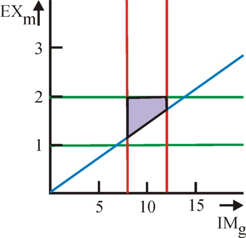
Figure 3: Boundaries for foreign trade
(export versus import, period 1)
(12) pB† · EX ≥ 0
In the formula 12 pB is the price vector in foreign currency.
The balance of the goods does not enter into the target function. It merely influences the value of the target function, as a consequence of the removal of the export products from x(t).
As an illustration an example of foreign trade is analyzed. The data of the economic system are taken from the previous paragraph (about the technique), for the situation where the production of corn and metal is done with only the first technique. Besides it is assumed that only metal is exported, and corn is imported. For reasons of notation the variable IMg = -EXg is defined. Since the balance for corn yields a deficit, IMg must be a positive number. Suppose that the state chooses the following boundaries: 8 ≤ IMg ≤ 12, and 1 ≤ EXm ≤ 2. The foreign price ratio is pmB / pgB = 7, just like in the domestic markets. The figure 3 shows the imposed boundaries for the (IMg, EXm) plane.
The LP probleem obtains for the first period (t=1) the form
(13a) -0.0833×xg + 2.29×xm − IMg ≤ 10.5
(13b) 0.5167×xg − 0.1048×xm + EXm ≤ 12.37
(13c) IMg − 7 × EXm ≤ 0
(13d) EXm − xm ≤ 0
(13e) IMg ≤ 12
(13f) EXm ≤ 2
(13g) IMg ≥ 8
(13h) EXm ≥ 1
(13i) xg + 7 × xm → max
The optimization requires the use of the simplex method, because four variables need to be determined. The result turns out to be [xg, xm, IMg, EXm] = [22.81, 10.65, 12.00, 1.714]. If this is compared with the situation without foreign trade, [xg, xm] = [25.1, 5.50] (see figure 1), then it is striking how the foreign trade increases the wealth. The import of corn is maximal (see the formula 13e), and the export of metal is precisely sufficient for the acquisition of foreign currency in order to guarantee the equilibrium of the balance of goods.
The model in this column supposes that all means of production are employed during the whole length Δt of the time interval t. Knop draws attention to the fact, that this is not always the case12. Namely:
This problem can be remedied by replacing everywhere in the formula 8 the variable xi(t) by
(14) xi(t) = ui(t) × ξi(t)
In the formula 14 ξi(t) is the available production capacity in the branch i, and ui(t) is the part that is really active in production (u of utilize). Obviously the value of this coefficient of utilization ui(t) of the branch i lies between 0 and 1. If desired this can be represented by a diagonal matrix U with diagonal elements ui × δij. Then the formula 14 gets the form x(t) = U(t) · ξ(t). If during the time interval new production capacity G · Δξ(t) is added, then the new extra capacity will not change in the next periods (apart from the discarded equipment). But its coefficient of utilization u(t) can very well take on a different value in each period13. The possibility of idle production capacity makes the model more realistic. Of course the necessary information needs to be collected, and the computations become more cumbersome.
In the real world a certain time τi will always pass between the placement of the order for new equipment of type i and its first productive use in the enterprise. For the equipment i must be produced, and subsequently be transported and installed at the location of the buyer and user. In other words, in all time intervals t, t+1, t+2, ... within the space of time τi there is a nett investment ii, that does not enlarge the stock (G · x(t))i = Σj=1N gij × xj(t) of the (active) fundamental fund in the branches j. The nett investments take away goods from the total product, but they do not immediately add new production capacity. The variable τ is called the delay or time lag of the investments. Eva Müller refers to the equipment in process of formation as the unfinished investments.
In the preceding columns it is usually assumed that τ is equal to the length Δt of a time interval t. Hans Knop rightly objects that this assumption is not in keeping with the practice. Dependent on the various types of equipment there is a large spread in the values of τ. If G · Δx(t) are the nett investments, which have been taken from the national income during the interval t, then a part will become available as productive capacity at the end of the interval t, a part at t + Δt, a part at t + 2×Δt etcetera. Therefore the netto investment is
(15) ii(t) = Σh=0H gij(t, h×Δt) × Δxj(t + h×Δt)
In the formula 15 H is the time horizon of the planning period. All investments are spread over a number of periods. The type of the investment in a certain equipment determines evidently the allotment and spread over the separate periods of the total investment sum.
In the formula 15 gij(t, h×Δt) are the time structure coefficients of the investments14. They describe how the equipment of type i will become productive in the branch j at a future time t + h×Δt. If one wants to perform a multi-period optimization, then the nett investments ii(t) couple the various periods in a sequence. Knop is here undoubtedly right, and in a model for practical application this must be taken into account. But the number of computations will increase to such an extent, that its application is beyond the scope of this column. Besides this type of refinements make it impossible to model situations elegantly with analytic equations. The application of numerical simulations becomes unavoidable.