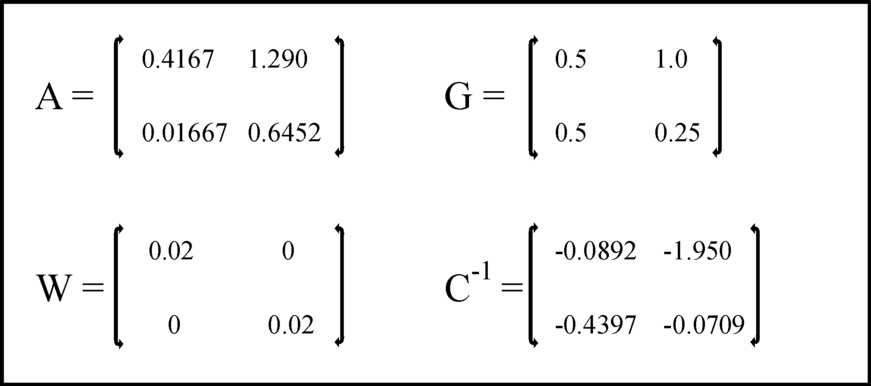
Figure 1: The elements in the matrices A, G, W en C-1
For the time being most columns on this internet portal concern the economic growth. The growth numbers determine to what extent the given social system has a veritable perspective for the future. That partly explains the interest of your columnist for the theories from the former Leninist states in Eastern Europe, that were competing with the west. The second-hand bookshop Helle Panke in Berlin is a goldmine for the acquisition of a small collection of books about central planning in the German Democratic Republic1. An asset from its stocks is among others the excellent book Volkswirtschaftlicher Reproduktionsprozeß und dynamische Modelle2, written by the economist Eva Müller. Here she presents in a clear way methods to calculate the material flow in a national economy or in a system of branches.
As soon as one really wants to take into account the economic structure, at the level of the branches, then it is necessary to resort to a model grounded on the intertwined matrix. Then the crucial task is to guarantee for a given technique of production, that the proportions of production between the branches remains balanced, and that there is no idle capacity of production. This is necessary, because the branches will commonly have divergent growth rates. In such an analysis the price system can yet be ignored. In an earlier column it is shown how Müller in her book works out the intertwined balance by means of the vector equation
(1) y(t) = (I − A(t)) · x(t) − i(t)
In the formula 1 the (vertical) vector x(t) represents the volume of production in the various branches, and the vector y(t) is the nett product, which is available for the consumptive purposes. The nett investments i(t) are taken from y(t), and are represented by the term F · ∂x(t)/∂t. This expression implies that the formula 1 is a first-order partial differential equation. The term A(t) · x(t) represents the material use during the production process. Müller calls it the material fund, in imitation of Marx. The term fund expresses that it is a permanent stock of goods. The model of the formula 1 is called the fundamental model of the dynamic intertwined balance.
The column just mentioned has already referred to the problem that the formula 1 with i = F · ∂x(t)/∂t ignores the existing fundamental fund itself (in the terminology of Eva Müller). The model includes only the additions to the material fund as a whole (circulation and fundamental fund together). The fundamental fund consists of the durable means of production, that are employed during the production process. They are the equipment, such as the machinery and the factory buildings, that wears away rather gradually. Marx calls her the fixed capital, and another common expression is the stock of capital goods. It is characteristic that she is not paid back with one productive revolution, but can be depreciated gradually (also called amortization). The depreciated equipment can be replaced by new equipment of the same type.
In the case of economic growth, of course the production can only proceed, as long as the fundamental fund also expands. In other words, the direct input of materials will increase, as well as the fund of fixed capital goods. Moreover the fundamental fund in each branch will have its own growth rate. Besides the expansion of the existing fundamental fund it must be guaranteed that all equipment is employed up to her maximum capacity. In the case of idle equipment there is an excess capacity. She has at least two disadvantages. First, less is produced than is allowed by the available capacity. In that situation the social wealth is not optimal. Second, the idle equipment does become obsolete, and therefore loses a part of her value, which is not regained by the sale of products.
In other words, the ecomic growth path must be chosen (planned) in such a way, that all existing capacity is used in an optimal manner. This is an important condition, besides the condition of an optimal consumptive offer3. Therefore it is desirable that the theoretical model of the dynamic intertwined balance explicitely takes into account the stocks of equipment (the fundamental fund). Eva Müller explains in her book methods to build such a model, and ways to solve it4.
This new model (according to Müller it has been developed by F.N. Klozwog, in the Soviet Union) features an extended investment equation. Both the replacement of equipment and the nett investments are modelled separately. Together they form the gross investments. In mathematical terms the separation is
(2) i(t) = iV(t) + iN(t)
Evidently the investments iV(t) for replacements must grow together with the volume of production. For each machine put out of use a replacement must be available. The nett investments iN(t) are made in order to enlarge the production capacity, and thus increase the volume of production. In principle the extension can consist of modernized machines.
Contrary to the model in the previous column now the extension of the circulation fund is not included in the investments i(t)5. Here Müller follows the definition of investments, that is common in western economics. Of course a growing economy does require an increasing circulation fund for each productive revolution. In the model the required material is withdrawn from the nett product y(t). In other words, in this case y(t) is not merely consumptive. Evidently the withdrawal is only possible as long as y(t) itself increases together with the economic growth.
The preceding column summarizes in a footnote the quantities, that are defined by Müller in order to describe the fundamental fund. That summary is repeated here, and elaborated in detail. The input of the required fundamental fund is given by the vector
(3) Γ(t) = G(t) · x(t)
In the formula 3 the matrix gij(t) indicates for each branch j the amount of product i that is needed as the fundamental fund. Note that in case that the nett investments lead to the addition of new equipment to the fundamental fund, the composition of the fundamental fund in a branch may change. The newly added equipment is as it were characterized by the matrix for that particular moment. Therefore G(t) in the formula 3 is written as a time dependent quantity. It is practical to compare the input Γi of the fundamental fund with the total production xi. In other words, define also the variable γi = Γi / xi. Müller calls the measure γi the intensity of the input of the fundamental fund6. Incidentally the intensity of the input of the fundamental fund is not really necessary for the present model.
Now it is possible to model the replacements iV(t) in the extended investment equation. The model with extended investment equation uses discrete time steps. Note that in this respect it differs from the previously described fundamental model of the dynamic intertwined balance, which yields continuous solutions7. In a discrete model t actually denotes the number of the period, that is analyzed. Each period has a duration Δt, so that the period t refers to the time interval between (t-1) × Δt and t × Δt. The discrete model yields as its solution for the period t the quantities like x(t). Since the period t has a duration Δt, the model implies that x(t) does not change during this interval. This is evidently only an approximation of reality (and of the continuous solution). The approximation will not cause large deviations from the true solution, at least as long as sufficiently small steps Δt are used.
Evidently the stock of the fundamental fund must already be available at the start of each production period. It is collected during the previous period. That is to say, Γ(t-1) is the stock, that will be used during the period t. At the start of the period t it is known that in each branch i a part of the equipment will be put out of use, due to wear. The corresponding rate of removal is represented by the symbol wi(t). In the model it is assumed that all removals are replaced. Then the rate of removal and the rate of replacement are identical. Naturally the replacement occurs at the time t, that follows t-1. Apparently the replacement investments are iV,i(t) = wi(t) × Γi(t-1). As usual, Müller transforms this equation into a matrix equation. That can be done by defining the diagonal matrix W in such a way, that she has the rates of replacement wi on her diagonal, and zeros elsewhere. In the mathematical notations this is wi × δij, where δij is the Kronecker delta. The result is
(4) iV(t) = W(t) · Γ(t-1)
Now the task remaining is to determine the nett investments iN(t), which must bring about the growth. The nett investments are simply the capital goods, that at the time t are added to the stock of capital goods (the fundamental fund). The discretization in the model implies that iN(t) is constant during the time interval Δt of the period t. Its size is approximated in the following way:
(5) iN(t) = (Γ(t) − Γ(t-1) ) / Δt
For the sake of convenience Δt is made equal to one unit (hour, day, week, month, year). In other words, one has Δt = 1. In an iterative (dynamic) calculation Γ(t-1) is known from the preceding iterative step at time t-1. However, the size of Γ(t) is still unknown at the time t. She is given by the formula 3, so that the formula 5 changes into
(6) iN(t) = G(t) · x(t) − Γ(t-1)
Now the model equation for x(t) can be derived. The formulas 1, 2, 4 en 6 are combined into
(7) y(t) = (I − A(t)) · x(t) − W(t) · Γ(t-1) − (G(t) · x(t) − Γ(t-1))
A rearrangement of the terms in the formula 7 yields the result
(8) y(t) = (I − A(t) − G(t)) · x(t) + (I − W(t)) · Γ(t-1)
The symbol I represents the unity matrix. This is the formula for x(t) in the model with an extended investment equation8.
This model can be solved with a fairly simple method. Rewrite the equation 8 as
(9) y(t) = C(t) · x(t) + D(t) · Γ(t-1)
In the formula 9 one has
(10a) C(t) = I − A(t) − G(t)
(10b) D(t) = I − W(t)
The solution of the formula 10 is
(11) x(t) = C-1(t) · y(t) − C-1(t) · D(t) · Γ(t-1)
The matrix C-1(t) is the inverse of the matrix C(t). In this model the development of the consumption y(t) is prescribed by the central planning agency. Of course the agency wil generally prefer a consumptive growth. Moreover in the beginning it has already been statd, that the "consumption" is also used for the growth of the circulation fund. Besides in the introduction it is pointed out, that the growth path must be compatible with the stock of the fundamental fund, that is present at the outset. The stock of the fundamental fund Γ(t-1) is known from the previous period, where it has been calculated with the formula 3.
The example takes over as much as possible the numbers, that have been used in the calculation with the fundamental model of the dynamic intertwined balance. So again the economic system with two branches is chosen as an example. The first branch is the agriculture, which concentrates on the production of corn (measured in bales). The second branch is the industry, and she produces metal (measured in tons, that is to say, 1000 kg). Both branches use a part of the produced corn and metal for themselves as the means of production (in the form of seed, fuel, tools, and the like). Obviously each of the two branches employs workers, Their wage is paid in bales of corn (for bread, gin etcetera) and in tons of metal (for domestic appliances etcetera).
In the model with the extended investment equation the two equations of the formula 8 must be solved. The solution is given by the formula 10. Here one must know the required funds A and G, which describe the state of the technology. Moreover the rates of replacement in W must be known. As the initial condition the stock of the fundamental fund Γ(0) at the time t=0 must be given. And of course the planning agency must prescribe for each period the consumptive offer y(t), that it wishes to realize. It will be clear, that the planning agency can not improvise at will, because naturally the available fundamental fund and the technology put certain limits on the possibilities for y(t).
In the example all matrices are taken constant in time. The matrix A is simply copied from the calculation in the column about the fundamental model. For the sake of completeness it is displayed again in the figure 1. A time independent matrix G implies, that the structure of the stock of the fundamental fund does not change by the nett investments. So the nett investments are characterized by the same structure as the existing fundamental fund. For the sake of convenience the matrix G is chosen equal to the matrix F, that is already known from the calculation with the fundamental model9. The rates of replacement w1 and w2 in the matrix W are both set to 0.02 (2%). Also G and W are displayed in the figure 1, just as for the sake of completeness C-1.
The initial conditions for Γ are chosen equal to [Γg(0), Γm(0)] = [11.6, 12.7]. The development of the nett product is fixed for all times to [yg(0), ym(0)] = [1, 0.3], with a time independent growth factor of 1.1. That is to say, the planning agency strives for
(12) y(t) = 1.1t × y(0)
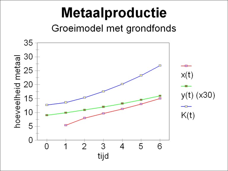
Figure 2b: The growth curves xm, ym (×30) and Γm for metal
Then the nett product, and with it the incomes, grow with 10% per time unit. Thus all data are available for the calculation of the desired development of the total social product x(t).
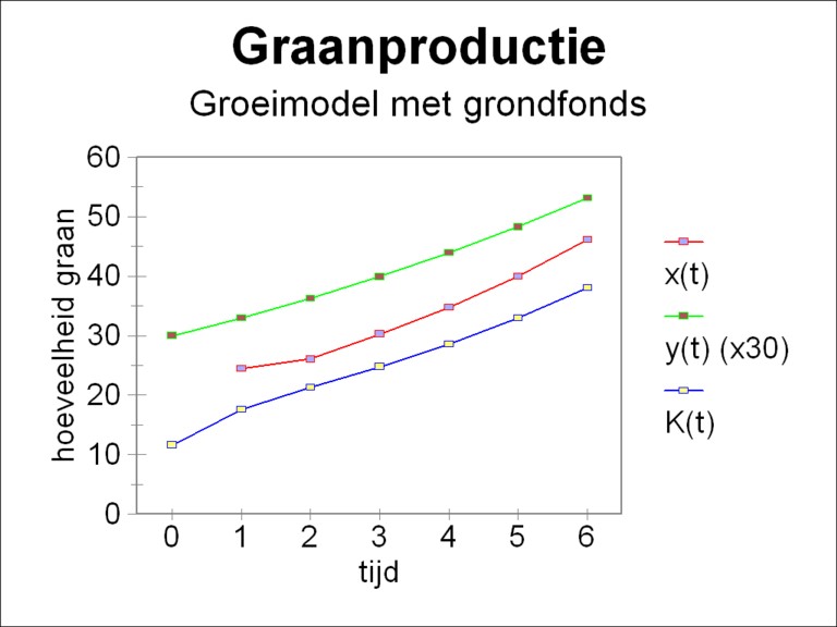
The calculations have been done for six consecutive periods t. The quantities x(t), y(t) and Γ(t) have been determined by means of respectively the formulas 11, 12 and 3. The figure 2a-b shows the results, where for the sake of clarity y(t) has been scaled up with a factor 30.
It is striking that the stock of the fundamental fund grows faster than the consumptive offer. In the first periods the investments are mainly directed towards the expansion of the fundamental fund in the agriculture. Thereafter both the agriculture and the industry grow with approximately 15.5% per time step. Due to the formula 3 the stock of the fundamental fund has about the same growth rate. A part of the production is used for the replacement of worn out equipment. The investments for the replacement occur at the cost of the nett investments, so that the growth in this model is slightly slower than in the simulation with the fundamental model. However, this effect is not very clear here, because the rate of replacement of 2% is rather small.
The fast growth of the total product x(t) and of the fundamental fund have as a consequence that an ever larger part of y(t) must be employed for the expansion of the circulation fund10.
The remaining part of this column discusses an improvement of the numerical algorithm in the model. This improves the accuracy of the model, but it contributes little to the economic insights. So readers, who are only interested in the economic aspects of the model, can safely skip the remainder. The numerical problem occurs in the formula 5, where the nett investments iN(t) are approximated by keeping its value constant over the entire time interval Δt. Due to this assumption the formula 5 follows in a logic manner from the general definition of the stock of the fundamental fund
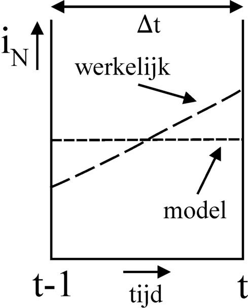
Figure 3: iN in model
and in reality
(13) Γ(t) = Γ(t-1) + ∫0Δt iN((t-1)×Δt + τ) dτ
But in reality the economy grows in a continuous way, so that the producers will generally also increase the nett investments. The figure 3 shows the real and modelled development of iN between (t-1)×Δt and t×Δt. In accordance with the integral formula 13 the surface under both curves is equal, namely Γ(t) − Γ(t-1). Here it is clear, that at the time t the real nett investments are larger than the modelled ones. In the model the investments are partly shifted towards an earlier time, closer to t-1.
The numerical results can be improved by a provisional correction of the discretization to the modelled nett investments. Eva Müller proposes to scale up the approximation (Γi(t) − Γi(t-1)) / Δt, which is too small, with a factor ηi 11. Evidently one has ηi > 1 for all branches i. The size of η is chosen on the basis of intuition and experience. It would be ideal to dispose of an exact analytical solution for x. Then the factor η is found simply by making the numerical solution coincide with the exact one. Just like has been done for wi and the matrix W also the scale factors ηi can be represented by a diagonal matrix, which is called J here. Eva Müller calls her the matric of the conversion coefficients. Then the formula 5 gets the form
(14) iN(t) = J(t) · (Γ(t) − Γ(t-1))
Of course the matrix J also affects the other formulas. The formula 8 for x(t) in the model with an extended investment equation changes into
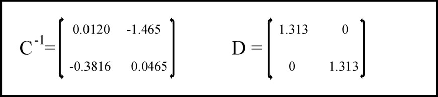
Figure 4: The elements in the matrices C-1 and D
(15) y(t) = (I − A(t)) · x(t) − W(t) · Γ(t-1) − J(t) · (G(t) · x(t) − Γ(t-1))
Now the formulas 10a-b change into
(17a) C(t) = I − A(t) − J(t) · G(t)
(17b) D(t) = J(t) − W(t)
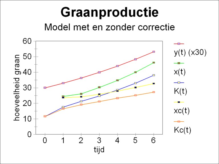
Figure 5: yg (×30), xg, Γg and, after correction, xg,c en Γg,c
In case that the formula 16 of Müller is preferred for Γ(t), then it can be employed in an iterative manner, such that Γ(t-1) is expressed as a function of Γ(t-2), Γ(t-3), ... , Γ(0).
The economic conditions in the example just studied are calculated again, but this time using the conversion coefficients η and the formulas 3, 11, 12 and 16a-b. Following Müller η = 1.333 is chosen for both branches and for all times12. The figure 4 shows the elements of the matrices C-1 and D. The figure 5 shows for the agriculture the results of the improved computation method, together with the original results. The results in the industry give a similar picture.
Of course the behaviour of the nett product y(t) is exactly identical to the figure 2a-b. The growth is still 10%. But now the growth of the stocks of the fundamental fund goes on in a slackened way, in comparison with the figure 2a-b. For in the later periods the growth rate of the stocks of the fundamental fund is only 8.3%, so even smaller than the rate for the consumptive offer. It is very striking, that due to the correction for the nett investments the total social product x(t) is clearly reduced.
The reason for the change is obvious. Due to the conversion coefficients the nett investments i(t) in the formula 1 now have their real size. The growth of the stock of the fundamental fund just prior to t is enlarged (and thus just after t-1 it is diminished, see the figure 3). In that way the required level of investment can be reached with a smaller social product. Müller finds the same results in her calculations.