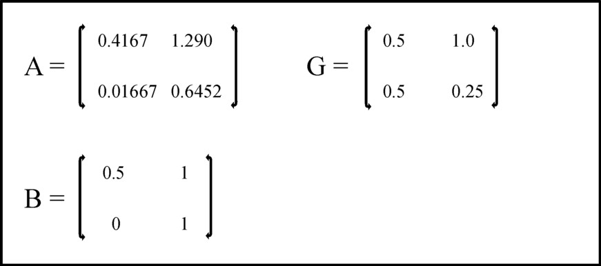
Figure 1: The elements in the matrices A, G and B
The book Volkswirtschaftlicher Reproduktionsprozeß und dynamische Modelle by the East-German economist Eva Müller is a goldmine of fascinating models, with a surprising diversiy. Here one finds keynesian growth models, next to input-output (Leontief) models, and three-sector models after the manner of Marx. But she also presents linear programming and optimization problems. The present column discusses her approach of those types of problems.
In the contemporary economic science linear programming and optimization problems are incorporared into the disciplines operations research, management analysis or production theory1. The application at the level of macroeconomics seems less useful, because the state has little control over the private production. In the former East-European planning economies the situation was different, and there linear programming was often applied. It was even invented and developed there2.
Linear programming (LP) is characterized by four properties3:
In case that there are only two decision parameters x1 and x2 the problem can be solved in a graphic manner. Then the limitations are lines, which restrict the area of possible combinations (x1, x2). The target Z is represented by a line, that must be shifted away from the origin as far as possible. The optimal solution will lie on the border of the restricted area. Incidentally, the most popular way of solving is is the so-called Simplex method4. The situation becomes more complicated, if the problem is dynamic. Then the factor time t add an extra degree of freedom to the problem.
The formulation of the LP is called the primal. Of course the reason is, that also a dual exists. For instance the primal can search for the optimal quantity of product, that can be generated in a given situation. Then the dual will search for the minimal production costs, as a sum of money, that must be covered under the given conditions of production. The formulation of the dual has the following characteristics5:
The starting point of Eva Müller, and thus also of this column, is the model of the dynamic intertwined balance with an extended investment equation6. In the column mentioned just now the following formula has been derived:
(1) y(t) = (I − A(t) − G(t)) · x(t) + (I − W(t)) · Γ(t-1)
The formula 1 is a matrix equation, with one row for each productive sector. The relation depends on time, with the variable t, because the dynamics is modelled for the whole duration of the economic plan. The vector x(t) is the total product, y(t) is the national (nett) product, minus the investments, and Γ(t-1) is the stock of capital goods (fundamental fund) in the period, immediately preceding the time t. The matrices A, G and W are respectively the use of material in the production process, the use of the fundamental fund, and the replacement of the fundamental fund. The symbol I represents the unity matrix. The vector Γ(t) is given by G · x(t). The reader can find a thorough discussion in the mentioned column.
The goal of the economic plans at the macro-level is the optimization of the consumption of the households. In the preceding columns that consumption is commonly put equal to y(t). In the model of the multiperiod optimization the approach is slightly different. Now it is supposed that one has
(2) (I − A(t) − G(t)) · x(t) + (I − W(t)) · Γ(t-1) ≥ y(t)
The formula 2 states that the output of the production process may exceed the nett product y(t). The planning agency chooses y(t) as the required minimum, but she does not object to quantities that exceed the plan. For instance the goals could be exceeded due to an economic use of the means of production, or due to funds which were not expended in the previous period. In this way the nett product is interpreted as the minimal level of consumption, that must absolutely be realized.
The formula 2 can be described succintly as a LP problem:
(3a) C · x(t) ≤ c(t), where
(3b) C = A + G − I
(3c) c(t) = Γ(t-1) − y(t)
For the sake of convenience Müller ignores here the replacements and the discarded equipment, which are embodied in the matrix W. It is assumed that the other matrices do not depend on the time t. For according to the requirement 4 above the problem must be linear.
The LP problem can be completed by the inclusion of additional limitations:
(4) B · x(t) ≤ b(t)
In the formula 4 B is a matrix, and b(t) is a vector which expresses the restrictions. The modeller can apply the formula 4 according to his own requirements. For instance the limitations can be dictated by the number of available workers, or by the scarcity of certain raw materials.
It has already been remarked that the goal takes on a particular form
(5) Z(T) = Σt=1T d† · x(t)
in the formula 5 Σ is the well-known mathematical symbol for summation, in this case over all periods until the planning horizon T. The symbol † indicates the transposition of d, which thus becomes a horizontal vector. The formula contains the inner product of d and x. In this LP the target function Z must be maximized. The vector d contains the weighing coefficients di for the product in each sector i. These coefficients are subjective. The differences in weight per sector express the intention to make some sectors grow faster than others. They symbolize the needs, that are felt by the consumers and/or the producers. The total value of the target function Z(T) has no further economic meaning.
The LP problem can be simplified further. For each time period t the target function can be maximized separately, so that there are T target functions with Z(t) = d† · x(t). And the matrices C and B in the formulas 3 and 4 can be combined into a single matrix M, just as the vectors c and b can be combined into a single vector m. It follows that:
(6a) M · x(t) ≤ m(t)
(6b) Zd(t) = d† · x(t)
Conformably to the recipe, that was given before, the dual problem is now:
(7a) M† · p(t) ≥ d(t)
(7b) Zd = m† · p
The dual target function Zd must be minimized. The vector p represents the weights for the quantities, which appear in the model. Note that among them are also quantities, which are not produced, namely in the inequality 4 the scarce raw materials, labour, etcetera. The minimization guarantees, that the cost for the production are minimal.
This example employs the same numbers, that have been used previously in the column about the intertwined balance with dynamic investment equation. For those are familiar to the reader. Besides, this approach illustrates the conseqeuences for economic growth, that result from scarcity. There are two sectors, so that the problem is two-dimensional. This has the advantate, that the situation can be portrayed well in a graph. The figure 1 shows the elements of the matrices A, G and B. The values of the coefficients in the matrix B have been chosen more or less arbitrarily.
The initial conditions for Γ are [Γg(0), Γm(0)] = [11.6, 12.7]. In the following the corn- and metal-indices are replaced by respectively the numbers 1 and 2. The nett product y and the restriction b due to the scarcity of resources (raw materialis, labour, valuta, etcetera) are on t=0 respectively [1.0, 0.3] and [13.5, 5.0]. Here b is chosen more or less arbitrarily. These two vectoren both have a growth factor of 1.1. That is to say, one has
(8) vector(t) = 1.1t × vector(0)
Finally the weight d in the valuation of the target function is set to [1, 1], because your columnist believes that corn and metal are equally important. In this way everything is ready for the formulation of the LP problem, and for solving it.
It may help to write down the LP problem for the first period (t=1) explicitly:
(9a) -0.0833×x1 + 2.29×x2 ≤ 10.5
(9b) 0.5167×x1 − 0.1048×x2 ≤ 12.37
(9c) 0.5×x1 + x2 ≤ 14.85
(9d) x2 ≤ 5.5
(9e) x1 + x2 → max
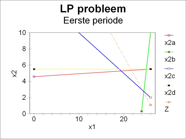
The figure 2 shows the region of allowed values for x. The legend shows which restrictions 9a-d correspond to the depicted lines. It turns out that for the moment the inequality 9d is not an extra restriction. Together the restrictions of 9a-c form a pentagon with its angles at the points [0, 0], [0, 4.59], [19.14, 5.28], [24.47, 2.62] and [23.94, 0]. The dotted line represents the target function Z. It touches the pentagon in the point [24.47, 2.62], and thus this is the solution of the problem. Here the target function reaches its maximum value of 27.08.
Compare the optimum found here with the product values, that in the earlier column about the intertwined model with an extended investment equation have been reported for the first period, namely [x1(1), x2(1)] = [24.5, 5.38]. Apparently the scarcity of resources (inequality 9c) slows down the economic growth, here notably in the second sector. Besides in the present LP problem the second sector causes a limitation (inequality 9b): his complete production is neede in order to realize the planned nett product. On the other hand the first sector realizes a large surplus, namelijk 6.55. Its cause is of course the small production volume in the second sector.
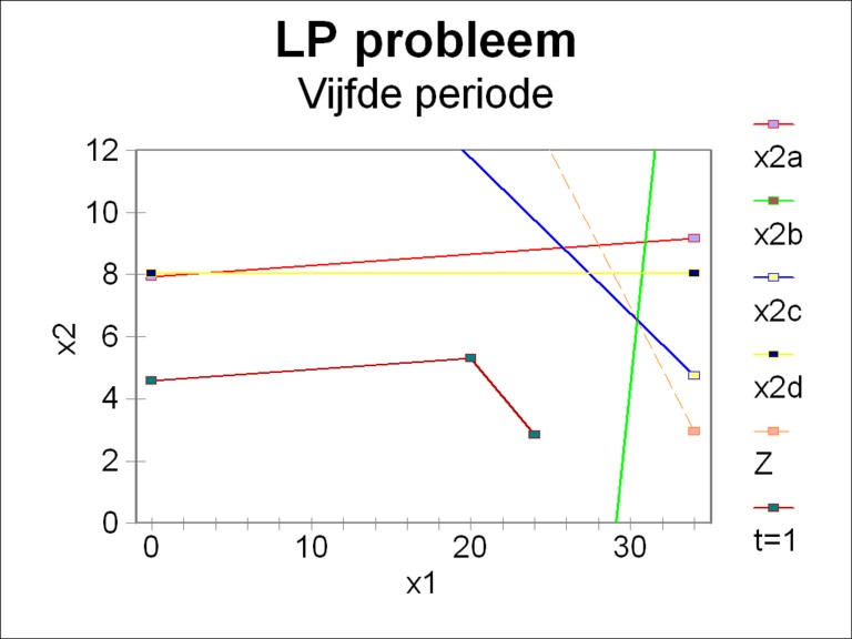
In the same way the LP problem can be solved for the next periods. In this example this has been done up to and including the fifth period. As an illustration the figure 3 shows for the fifth and last period the region of allowed values. For comparison also the pentagon of the period 1 has been depicted. First of all, it is striking that meanwhile the allowed region has become a hexagon. Namely, already since the second period also the inequality 9d is relevant. Furthermore it is striking that together with the growth of the economic system also the size of the region of allowed values increases. In all these periods the optimal point remains the intersection of the lines 9b and 9c. In the fifth period the maximal value of the target function Z has risen to 36.94.
For the sake of completeness the table 1 shows for all five periods the values of the essential quantities. Due to the scarcity of the first resource, which is imposed by the inequality 9c, the size of the second sector is squeezed. Thus the first sector produces a surplus for all periods. The central planning agency could consider to use that surplus for a higher consumption. Then the nett product is simply the minimla consumption level, that must be realized. And although the inequality 9d is definitely relevant, she is apparently not a bottle-neck in any of the periods. On the contrary, a part of this second resource is permanently unused.
| Periode | 1 | 2 | 3 | 4 | 5 |
|---|---|---|---|---|---|
| x1 | 24.47 | 25.03 | 26.28 | 28.08 | 30.41 |
| x2 | 2.61 | 3.83 | 4.83 | 5.73 | 6.53 |
| Surplus 1 | 6.55 | 6.97 | 6.13 | 5.73 | 5.73 |
| Surplus 2 | 0 | 0 | 0 | 0 | 0 |
| Unused 1 (9c) | 0 | 0 | 0 | 0 | 0 |
| Unused 2 (9d) | 2.89 | 2.23 | 1.82 | 2.32 | 1.52 |
The formulas 7a-b represent the dual problem of the formulas 6a-b. In the first period of the present example the formulas 9a-e change into the dual form:
(10a) -0.0833×p1 + 0.5167×p2 + 0.5×p3 ≥ 1
(10b) 2.29×p1 − 0.1048×p2 + p3 + p4 ≥ 1
(10c) 10.5×p1 + 12.37×p2 + 14.85×p3 + 5.5×p4 → min
This LP problem can not be solved in a graphic manner, because it contains four dimensions. Nevertheless it is fairly simple to obtain a solution, namely by means of the simplex method. She gives a step-by-step recipe that manipulates the set 10a-c in such a manner, that only the essential quantities remain. Comprehension is not required, and this saves a lot of headache. For details the reader is referred to the introductory textbooks7. The application of the method yields as a result p = [0, 0.8786, 1.092, 0] 8. It can be immediately verified, that the target function Z has the same optimal vale as before in the primal problem9. The elaboration of the dual for the next periods requires a persistent calculation, and is left as an exercise for the reader (if he or she feels the urge).
The quantities p are interpreted as the opportunity costs of the two products and of the two resources. Yet another name is shadow prices. They indicate the change in value of the target function Z, when a unit of product or of a resource is added to (or removed from) the system. The weighing coefficients di in the formula 5 determine the shadow prices. In the present example one finds d = [1, 1].
Eva Müller gives the following interpretation of the dual result10. There is a surplus of product in the first sector, and a surplus of capacity for the second resource. They impose no limitation on the growth, and therefore an additional unit is worthless. That is to say, their opportunity costs equal zero. On the other hand the second sector can only just meet the requirement for the nett product (minimal consumption level), and the first resource is used completely. If one succeeds in realizing their expansion, then a further growth of the nett product becomes possible. In that case the (optimal) value of the target function will increase. It has already been noted that the shadow prices indicate the expected rise in value.
In the west there is a lot of literature with regard to linear programming. However, it is applied only at the micro level, often in order to maximize the profit of the firm. It is interesting and original to see in the book by Eva Müller an application at the macro level. And it yields a tangible insight into the effect that the scarcity of resources has on the growth perspectives within the society. One wonders what the capitalist states miss, by neglecting this discipline of economics at the macro level.