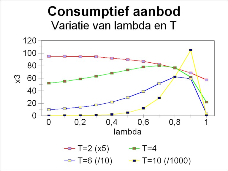
Figure 1: consumption x3 for various λ and T
G.A. Feldman is a Russian economist, who has contributed significantly to the development of the modern theory of planning. In the west his work is hardly known, probably for ideological reasons. Thus the information in this paragraph originates from a book by a Russian economist, namely I.M. Osadchaia2. In fact Feldman elaborates on the theory of the two-sector models, that in the nineteenth century has been proposed by K.H. Marx. In 1928 Feldman publishes his most important article, On the theory of the rates of the national income, in the magazine Planowoje chosjaistwo.
In imitation of Marx, Feldman tries to describe the structure of the economic system. It is true that for society in the first instance only the growth of the national income (the nett product) is relevant, but this is closely related to the development of the stocks of the material funds. Therefore Feldman designs a theory, where both the department II for the production of the consumption goods, and the department I for the production of the means of production, are present. So the department I extends the production fund (fundamental fund, the stock of capital goods). Suppose that the stocks of the fundamental fund in the departments I and II equal respectively gI and gII. Then the structure of the economic system is determined by the coeffient ιk = gI/gII. This is the primary index of the system.
The value of the index ιk has a direct influence on the growth of the consumptive supply. Feldman advocates to make the departments I and II grow with the same rate of growth, that is to say, in proportion. However, he also mentions the option to change the structure of the economy, by a temporary additional extension of the investments in one of the departments. In this way the planned investments can steer the economy towards her optimal situation.
According to Osadchaia, Feldman studies the input of the factor labour in addition to the influence of the factor capital. Unfortunately Osadchaia does not elaborate on this point. In general this type of models assumes that the factor labour adapts naturally to the stock of capital goods. If the total product is x, an there are l workers, then they are supposed to have a labour productivity ap of x/l.
Osadchaia states, that Feldman is the first person to point to the need of a high efficiency of the fund. He defines this efficiency as k = x/g. Several decades later this idea is also introduced in the west, notably due to the work of the economists R.F. Harrod and E. Domar. As can be expected in the competition between power blocks, they give another name to the efficiency of the fund. Domar introduces her inverse, and he calls it the capital-output ratio3. Osadchaia remarks, that at least Domar was familiar with the texts of Feldman, and was inspired by him. Incidentally, note that the theories of Harrod and Domar are both one-sector models.
At first sight the present dynamic three-sector model has a close resemblance to the model of Biersack, that has been discussed in a previous column. However, the distribution of production over the three branches uses slightly different criteria, namely:
In comparison with the model of Biersack the present model has the evident disadvantage, that here the material flows are not modelled. The analysis is limited to the production of the consumer goods and of the investment goods. The structure of the total economy remains partly invisible, namely as far as the production of raw materials is concerned.
In the marxist reproduction schemes only the branches 2 and 3 are present. Perhaps this fact makes it surprising, that Robinson and Eatwell add the branch 1. In their vision it represents the heavy industry. The heavy industry manufactures equipment like large milling machines and rolling machines. And the branch 2 uses those machines for the manufacture of for instance plows and threshing machines, and sells them to the branch 3. So mainly the branch 1 allows the branch 2 to replace its worn-out equipment with new ones. Without the branch 1 the production capacity of the branch 2 would slowly diminish. As long as the branch 1 supplies sufficient machines, the branch 2 can even invest and grow in size. This raises the obvious question whether the branch 1 can invest for itself. In the model this is solved by letting the branch 1 manufacture its own investments.
This model of Feldman has the merit that it illustrates better yet than the dynamic three-sector model of Biersack how important the decisions about investments are. For the branch 1 must judge all the time, whether its production will be sold to the branch 2, or will be kept for its own investments. In the first case the shareholders of the branch 1 will enjoy a conspicuous dividend. And in the second case the branch 1 will make investments, and grow in size. The branch 1 could invest persistently so much, that the branch 2 would only be able to replace its worn-out equipment, or even not that. In that situation the production in the branch 2 will stagnate, and consequently also the production of the branch 3, while the branch 1 continues to grow. Apparently a total economic growth is conceivable, while yet the consumptive supply remains unchanged. Here and there new factories are built, whereas the people experience a steady welfare4.
The formalism in the model of Feldman is comparable to the one of Biersack. The coefficient of the efficiency of the fundamental fund is defined by
(1) ki(t) = xi(t) / gi(t)
In the formula 1 xi is the production of the branch i, and the quantity gi represents the stock of the fundamental fund in the branch i.
Robinson and Eatwell simplify their version of the model of Feldman, by omitting the scrapping of equipment. Then there is no need for replacements, the rate of replacement w equals 0, and all investments are available for the economic growth. This simplification has the advantage, that the model is somewhat more transparent. The obvious disadvantage is, that scrapped equipment can be a source of economic stagnation. If the scrapped equipment is ignored, then a bright scenario emerges, where the economy will inevitably grow.
The branches 1 and 2 both add equipment to the stock of the fundamental fund. Define Δgi(t) = gi(t) − gi(t-Δt), where t is the time variabele and Δt is a time interval. Then one has
(2) x1(t-Δt) + x2(t-Δt) = Σj=13 Δgj(t)
In the preceding paragraphs it has already been explained how the quantities Δgi(t) each separately are connected with the production xi. The mathematical expression of that argument is
(3a) x1(t-Δt) = Δg1(t) + Δg2(t)
(3b) x2(t-Δt) = Δg3(t)
The present version of the model of Feldman is characterized by the freedom of the producers in the first branch (or the central planning agency, which commands them) to choose their policy. They are free to determine the size of their investments as they think fit:
(4) Δg1(t) = λ(t) × x1(t-Δt)
In the formula 4 λ(t) can have any value from 0 to 1. Now it follows immediately from the formula 2 that one has
(5) Δg2(t) = (1−λ(t)) × x1(t-Δt)
In the dynamic three-sector models such as proposed by Biersack it is common to introduce three so-called steering parameters, which express how the investments i(t) = Σj=13 Δgj(t) are distributed among the three branches. These coefficients of the investment share are defined by
(6) ui(t) = Δgi(t) / i(t)
Of course this requires that u1 + u2 + u3 = 1, so that one of the steering parameters if fixed by the other two. Then the formulas 1, 2, and 5 can be combined in the equation
(7) Δgi(t) = ui(t) × (k1(t-Δt) × g1(t-Δt) + k2(t-Δt) × g2(t-Δt))
However, this method does not really make sense for the three-sector model of Feldman, because there the investments are mutually directly connected. There is just one steering parameter, namely λ(t). This single parameter is sufficient for the optimization of the performance of the economic system. A target function is chosen, and values for λ(t) are searched, that yield the largest possible value of the target function. The performance of the economy is always judged by an evaluation of the consumptive supply. Therefore a logical target function is
(8) ZI(T) = x3(T)
In the formula 8 T refers to the time, when the target function will be evaluated.
It is probably useful to point out, that a constant steering parameter λ does not by itself yield constant steering parameters u. It is clear from the formulas 3b, 4, 5 and 7, that u depends on (k1(t) / k2(t)) × (g1(t) / g2(t)). This factor is generally time dependent, even if the coefficients k of the efficiency of the fundamental fund would be kept constant.
Apparently constant values of u occur only, as long as the stocks of the fundamental fund in the branches 1 and 2 are and remain in proportion. That is the case for a constant k under the condition λ = g1(0) /(g1(0) + g2(0)). It is true that this is an important case, but in the model of Feldman it is not the most fascinating one. The interesting aspect in the model of Feldman is, that the paths of economic growth can be changed by improving the economic structure. Proportional growth is satisfying, as soon as the optimal structure and the optimal growth path have been reached.
The formulas 3b, 4 and 5 can be solved in an exact manner, if an infinitesimally small time interval Δt is taken. In mathematical terms this means Δt → 0. Then one has Δgi(t) = ∂gi(t)/∂t × Δt, so that the formulas 3b, 4 and 5 change into
(9a) ∂g1(t)/∂t = λ(t) × k1(t) × g1(t)
(9b) ∂g2(t)/∂t = (1−λ(t)) × k1(t) × g1(t)
(9c) ∂g3(t)/∂t = k2(t) × g2(t)
The model becomes better manageable, when the quantities k and λ are taken to be constant in time. Then the system of equations 9a-c has a simple solution:
(10a) g1(t) = eλ×k1×t × g1(0)
(10b) g2(t) = (1/λ − 1) ×(eλ×k1×t − 1) × g1(0) + g2(0)
(10c) g3(t) = (1/λ − 1) × k2 × ((eλ×k1×t − 1) / (λ × k1) − t) × g1(0) + k2 × g2(0) × t + g3(0)
The formula 10c illustrates clearly the development of the stocks of the fundamental fund. At t=0 the third branch starts with a stock at the size of g3(0). The branch 2 starts with its stock at the size of g2(0), and in each time unit that stock provides the third branch with a quantity x2(0) of new machines. At the same time the first branch is constantly adding machines to the stock of the second branch. And also those machines, added to the branch 2, again produce for the benefit of branch 3.
In the long run the ratio g2(t) / g1(t) approaches 1/λ − 1, and g3(t) / g2(t) approaches (1/λ) × k2 / k1. It must be remembered, that the analytic solution, that has been found in the column about the three-sector model of Biersack, is not applicable for the present situation. For u is time dependent.
An example is always clarifying, for those who strive for a feel with respect to the theory. In this example the initial conditions are chosen equal to the numbers of the economic system in the earlier column about the three-sector model of Biersack. when those numbers are converted to the present model, then one obtains x1(0) + x2(0) = 6.232, x3(0) = 1.1, g1(0) + g2(0) = 4.289, and g3(0) = 0.88. Moreover suppose that the stock of the fundamental fund in the second branch is twice as large as the stock in the first branch. That assumption results in g1(0) = 1.430 and g2(0) = 2.859.
Evidently it is convenient to use the analytic solution from the formula 10a-c. Therefore it is assumed that the efficiency of the fundamental fund k does not depend on time. Besides it is assumed, that the efficiencies in the branches 1 and 2 are identical (k1 = k2). Then the formula 1 yields the result k = (1.453, 1.453, 1.25). Furthermore λ is taken to be a constant for all times.
Now the optimization problem is tackled by using the continuous solution, that is described by the formulas 10a-c. The consumptive supply x3(t) = 1.25 × g3(t) merits a Special attention, because it determines the welfare in the society. The function ZI of the formula 8 at the time period T is choses as the target function, that is to be maximized. For the evaluation of precisely this target function requires only a few computations. The value of the time period T must yet be chosen. Apparently T itself is a part of the optimization problem.
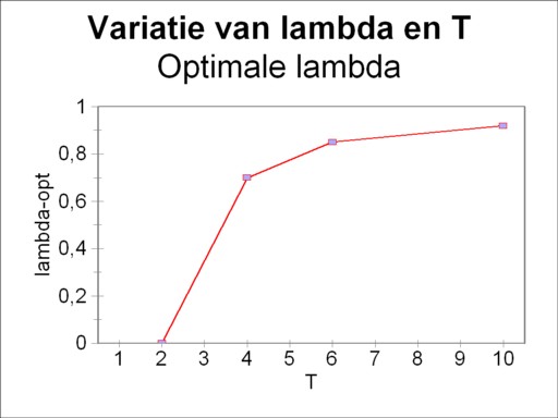
The interval of possible values for λ is [0, 1]. In this example the time horizon T is varied with corresponding values T=2, 4, 6 and 10. The results of the variation calculus are shown in the figure 1, with along the vertical axis the target function ZI and thus also the consumptive supply x3(T). Note that x3 is scaled for T=2, 6 and 10, so that all curves are clearly visible in the same figure5. The shapes of these curves remind of the curve, that has been found with the model of Biersack. Its explanation can also be found in that column. The figure 1 shows clearly, that the optimum of the target function shifts towards higher values of λ, according as the time horizon is shifted towards the future. For the sake of completeness this behaviour is shown in the figure 2.
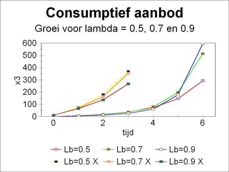
It is true that the figures 1 and 2 indicate the values of the steering parameter λ, which yield the largest consumption possible, but they do not say why. It is clarifying to illustrate also how the growth of x3 develops with time. Therefore in the figure 3 the curves x3(t) are drawn for λ=0.5, 0.7 and 0.9. Since at the beginning the behaviour is not clearly visible because of the vertical scale, for the sake of convenience the curves in the interval [0, 3] have also been magnified by a factor 10. In the magnified time interval the economic system with λ=0.5 gives the best results. The systems with λ=0.7 and 0.9 have a slow start, as it were. For t=4 and 5 one prefers λ=0.7, and thereafter λ=0.9. Incidentally your columnist shows the figure 3 also, because such nice growth curves should not be absent in a column like this.
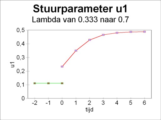
In this example the proportional growth occurs for λ = 1/3. If the optimal λopt exceeds this value, then apparently an economic structure is needed with relatively more equipment in the first branch. The weight of the branch 1 in the economy should increase, until the new proportions, belonging to λopt, have been reached. In addition the weight of the branch 2 with respect to branch 3 will increase. In that transitional situation the steering parameters u change continuously, and will finally in the long run stabilize on their new equilibrium value. This phenomenon is illustrated in the figure 4, where at the time t=0 a transition is made from λ = 1/3 to λ=0.7. The steering parameter u1 makes a discontinuous upward jump, and thereafter approaches its new equilibrium value6. The steering parameters u2 and u3 exhibit a similar behaviour, however in the present example with a downward jump and downward adaptation7.
A question remains to be answered: why does λopt in the figure 2 increase for a time horizon T farther away in the future? Consider the following two more or less extreme situations of optimization:
It is probably good to stress again that the three-sector model of Biersack can not provide any information about such aspects. In the model of Biersack all producers of the means of production are united within one single branch, both the heavy and light industry. In that model it is impossible to extend for instance specifically the investments in the heavy industry. That is to say, the model of Biersack does not install an industrial structure within the production of the means of production. It is one homogeneous group.
Another point worth mentioning concerns the target function Z. She defines what is optimal and what not. Therefore a completely different optimum will be found, when the target function is changed. For instance strictly speaking the target function ZII(T) = Σt=1T x3(t) seems a better choice. She is the sum of all consumptive supplies during the time period T. In this way also the interests of the people in the present will be taken into account. In the end the choice of the target function is a political decision. And consequently also the optimum itself remains a political decision.
It is worth while to reflect on the use of this kind of computations. The purpose of the model is of course to adapt the productive proportions in the economic system to the needs, and to optimize them. In an economy with central planning this development must proceed by means of a policy, based on political decisions. In a market economie with competition the desire for profit will introduce a certain degree of order. But also in that case the state posesses the means to intervene with rigour, if desired. For instance a certain new activity (metal industry, information technology, etcetera) can be built up rapidly by means of subventions or state enterprises.
The approach described just now changes the structure of the industry in a radical manner. It must be realized that this revolution has large consequences for the workers in the concerned branches and sectors. Some sectors are allowed have a durably faster growth, and the growth of others is slowed down. It is obvious that the planners must take into account the rebellion of the hurt economic branches. For the workers and the firms become aware, that they do not take part in the growth, which they observe elsewhere in the economy. That will certainly foster pessimism and a negative attitude. So it remains to be seen whether politics is able to restructure the economy.