One-sector models with scarce capital

First insertion on Heterodox Gazette Sam de Wolff: 24 march 2014

Two years ago this web portal discussed two dynamic one-sector models, which have been used in the planning activities of the former Leninist economies. In fact these are difference versions of the Harrod-Domar model, which use time dependent structure parameters. This makes the models completely dynamical. In the present column several planning instruments of the famous Dutch economist Jan Tinbergen will be explained, also based in the Harrod-Domar model. His planning models take into account the delays in investment and the replacements. They are copied from the book Mathematical models of economic growth, which Tinbergen has written in collaboration with Hendricus C. Bos¹.

The models try to solve the policy problems. The policy maker will formulate targets, which according to him will optimize the welfare. The welfare is mainly expressed by the average level of consumption, but also by the distribution of the consumption among the people². Often the planning is refined in steps, so that first the macro problem is solved. Then the problem at the micro level is solved in the next phase. It is common to optimize also the employment, besides the consumption.

Figure 1: Tinbergen coin Child right

Planning is necessary, even when the state does not directly intervene in the economy. The state levies taxes and spends the proceeds in order to perform its tasks, A part has the form of investments. Besides, some private activities are stimulated by means of subsidies. The aim of the macro-economic models is to eliminate possible conflicts and clashes from the political plans. Even in the first phase the savings-quote σ and the economic growth rate g_Y must be reconciled. This must precede the structuring of the branches. When the approach of Domar and Harrod is applied, then the capital coefficient κ is constant. In other words, for now the technological changes are ignored.

The models in this column merely describe one sector, namely the total economy as a whole. Since they are applied in the planning of the economic development, the time t is an essential variable. The structure of the economic system is fixed by means of general parameters, such as the mentioned σ and κ. The extent of the economic activities is determined by the value of the national income Y(t). For the sake of convenience it is assumed, that the stock of capital goods (with a value of K(t)) is the only scarce resource.

The economic growth requires an increase of the capital K(t). Therefore nett investments I(t) are made, which by definition equal

(1)     I(t) = ∂K(t) / ∂t

A common policy target is the equilibration of growth, apart from possible interim adaptations. This implies that the nett investments must be completely covered by the savings. In formula this is I(t) = S(t). Due to the definition of the savings-quote the savings equal

(2)     S(t) = σ × Y(t)

For the sake of completeness the reader is reminded of the definition of the capital coefficient:

(3)     κ = K(t) / Y(t)

The capital coefficient expresses the size of the stock of capital goods, which is needed for the production of a certain national income Y(t). Since κ does not depend on t, the growth is apparently extensive. In other words, K and Y are scaled up in proportion. The factor labour L(t) is absent in the formulas. It is assumed that the labour market will adapt in a flexible manner to the economic developments³.

In the preceding text it has already been stated, that the consumption C(t) is an essentieel element in the policy targets. She can be calculated directly from the formula of the national income

(4)     Y(t) = C(t) + S(t)

According to the formula 4 the consumptions of the households are paid from the national income. That part which is not consumed, is saved by the households. Next, due to the assumption S=I, the savings are also expended. This is done by the enterprises, who loan the sum S in order to buy capital goods (production equipment) with a total value of I.

The investments lead to an economic growth. A model can usually only produce an exact mathematical solution, when a constant growth rate is assumed, so independent of the time. For instance, the growth rate of the national income is defined as

(5)     g_Y = (∂Y(t) / ∂t) × dt / Y(t)

In the formula 5 the quantity dt is the time interval, which corresponds to the growth rate. For, according as the interval is longer, Y will grow more. It is common to equate dt to a single time unit. In the same manner the other growth rates can be defined, such as the one for K(t).

The formulas 1-5 are the foundation of the Harrod-Domar model. The model can be refined in various ways, depending on the questions, which arise during the planning process. The models, which will be discussed in the present column, are similar to the ones, which the Leninist economist Eva Müller in the mentioned column calls the simple national income model. The work of Müller does not refer to Tinbergen, although her book appears twelve years after Mathematical models of economic growth⁴. She does refer to Russian and East-German publications, but these also appeared several years after the book of Tinbergen. Nowadays is seems incredible, but perhaps Müller was really ignorant!

Model with investment lag

The planning process must take into account, that it takes time to realize the decisions. This concerns notably the investments. After the decision to invest the order must still be placed with the producer, and he will need some time to make and install the product. For, investments in capital goods are often large in size and commonly made to measure. This is certainly true for infrastructural works, which may take years to complete.

A realistic model must take into account this investment period or delay (lag). Suppose that the investment begins at the time t, and that it requires a period τ. Then the average investment per unit of time is⁵

(6)     I(t) = (K(t + τ) − K(t)) / τ

That is to say, at the time t the yearly payment must be made for all capital goods, which will be delivered between t and t+τ.

The combination of the formulas 2, 3 and 6 leads to a recursive relation

(7)     K(t+τ) = (1 + τ × σ / κ) × K(t)

From this formula the growth rate of the capital can simply be derived⁶

(8)     g_K = ln(1 + τ × σ / κ) / τ

In the formula 8 ln(x) is the natural logarithm of x, and the growth rate holds for dt=1. In case that τ is much smaller than σ/κ, the well-known formula g_K = σ/κ is found in a good approximation. When this is not the case, then the growth will be slower. The lagged delivery of capital goods slows down the growth.

Model with depreciations (1)

In this paragraph the effect of the wear of the capital goods on the growth is studied. Now for the sake of convenience it is assumed that τ=0, so that the investment lags are ignored. Suppose that a yearly quantity A(t) of capital goods is scrapped, whereas a quantity V(t) is added as a replacement. Suppose that the quantity Γ represents the value of the stock of capital goods. Then one has

(9)     ∂Γ(t) / ∂t = I(t) + V(t) − A(t)

Here the loyal reader recognizes the formula 9 as the equation for the fundamental fund in the simple national income model of Eva Müller. The other formulas of Tinbergen and Müller are also similar. Thus Tinbergen defines the average service life of the capital goods as

(10)     θ = Γ(t) / V(t)

Note that here θ is constant with time. Apparently the producer depreciates his stock of capital goods during a time θ, and uses the deprecations for the ongoing replenishment of the stock. The replacement V(t) compensates the part of the capital goods Γ(t), which in the future period θ will be discarded. Its goal is to maintain the production capacity. Depreciations are a part of book-keeping. Furthermore, note that the rate of amortization of Müller equals 1/θ.

The nett investments I(t) satisfy the formula 2, in combination with S=I. In other words, the savings behaviour does not depend on the scrapped goods. Therefore, ∂Γ(t) / ∂t will generally not equal I(t). Then, due to the formula 1, Γ(t) and K(t) will also differ. Apparently in this model K(t) must not be interpreted as the stock of capital goods, but as the stock of money capital, which results from the savings of the households. Note, that the formulas of Müller do take into account the lags in both the nett investments and the replacements. However, subsequently she still neglects those lags in her examples, because otherwise the computations would be to complicated.

In this model one has gross investments I_B(t). They are defined as

(11)     I_B(t) = I(t) + V(t)

The discarded goods A(t) do not equal the replacements V(t), because they relate to the past. Due to the lifetime θ the goods A(t) will equal the purchases at the time t-θ. Since those purchases are exactly the gross investments, one must have

(12)     A(t) = I_B(t − θ)

The formula 12 completes the model. Now a solution can be determined for the description of the economic growth. Tinbergem chooses a solution of the form

(13)     K(t) = K(0) × e^{gK × t}

Here g_K is the growth rate of the money capital. The substitution of the solution 13 in the formulas 1, 2 and 3 leads to the well-known relation g_K = σ / κ. Due to the formula 3 this also fixes the growth of Y(t).

Yet the state can not simply choose any savings quote in its political plan. Namely, the average lifetime θ of the capital goods affects the possibilities for growth. This can be shown by combining the formulas 9, 10, 11 and 12. The result is

(14)     ∂Γ(t) / ∂t = I_B(t) − I_B(t-θ) = (Γ(t) − Γ(t-θ)) / θ + I(t) − I(t-θ)

The formula 14 is a linear inhomogenous difference-differential equation. The theory of differential calculus (and previous examples on this portal as well) states that the solution consists of a general part and a particular part. In this case the general solution turns out to be zero⁷. Tinbergen proposes to try as the particular part Γ(t) = Γ(0) × e^{gK × t}. When this function is inserted in the formula 14, together with the formula 13, then the result is

(15)     g_K = { 1/θ + g_K×K(0)/Γ(0) } × (1 − e^-gK×θ)

The formula 15 can not be solved in an exact manner. However, the message is clear, namely that the equilibrated growth is determined by the initial conditions K(0) and Γ(0), and by the lifetime θ. Since for the savings quote one has σ = κ×g_K, the savings quote for equilibrated growth is also fixed in advance. There is no remaining freedom of policy choice, unless in advance a period of structural adaptation is inserted.

Model with depreciations (2)

Tinbergen rightly remarks, that for the case with depreciations it is not obvious to use the formula 3 ⁸. For, there the economic structure is related to the nett income Y(t). In the discussed model with an investment lag that is logical, because the nett income represents all newly added value. The value is completely available as an income, either as a wage or as a profit or rent. But in the model with depreciations a part of the newly added value must be reserved for the discarded goods V(t). To be precise, the newly added value Q(t) is divided according to

(16)     Q(t) = Y(t) + V(t)

Therefore it is better to define the economic structure by means of the constant

(17)     γ = Γ(t) / Q(t)

Tinbergen calls γ the gross capital coefficient. Eva Müller calls γ in her model with an extended investment equation the intensity of the use of the fundamental fund (where, as the loyal reader remembers, the fundamental fund is another name for the stock of capital goods). Thanks to the definition in the formula 17 all formulas from the preceding paragraph become a trifle more elegant.

Now find for the gross investments a solution of the form I_B(t) = I_B(0) × e^{gK × t}. When this is combined with the first equation of the formula 14, and subsequently the resulting differential equation is solved, then the solution is

(18)     Γ(t) = I_B(t) × (1 − e^{-gK × θ}) / g_K

Figure 2: g_K according to the formula 19

Besides, one now has I_B − V = I = S = σ×Y = σ × (Q − V) = σ × Γ × (1/γ − 1/θ), where all values pertain to the time t. Here rewrite V by means of the formula 10, then the following convenient formula emerges

(19)     g_K = (σ / γ + (1-σ) / θ) × (1 − e^{-gK × θ})

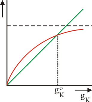
The formula 19 is a trifle more clear than its counterpart, the formula 15. When the parts of the formula 19 are interpreted as functions of g_K, then the lefthand side is a straight line through the origin, and the righthand side is a power of e, with as its horizontal asymptote σ / γ + (1-σ) / θ.

Apart from the trivial solution g_K = 0 the solution of the equation 19 is found as the intersection of the straight line and the asymptotic power of e. See the figure 2. For large values of θ the formula 19 reduces to the well-known form g_K = σ/γ. On the other hand, for small values of g_K × θ the power of e can be approximated by a Taylor series, which approximately yields the expression g_K = 2 × σ × (1/γ − 1/θ). Some solutions will consist of complex numbers. This means that they exhibit a cyclical behaviour⁹. They are irrelevant for the practice of planning, which is evidently interested in the tendency to grow.

An interesting aspect of the formula 19 is also the option to directly calculate the savings-quote:

(20)     σ = { g_K / (1 − e^{-gK × θ}) − 1/θ } / (1/γ − 1/θ)

Another peculiarity of this version of the model with depreciations is that the ratios K/Y, K/Γ and A/V are all independent of time. Thus the model gives a clear insight into the various developments. After some calculations¹⁰ one finds K/Y = σ/γ, K/Γ = 1 / (1 − e^{-gK × θ}) − 1/(g_K × θ), and A/V = g_K × θ / (e^{gK × θ} − 1).

It is instructive to consider two limiting cases, namely very small values of g_K × θ, and very large values of θ (and thus also of g_K × θ and of θ/γ). The results are summarized in the table 1. For small values the discarded goods and the replacements are nearly equal, because the situation hardly changes during the time θ. Then the money capital is half of the productive capital. On the other hand, for a very long lifetime the (future) replacements must be much larger in quantity than the scrapped goods. Then the gross capital coefficient γ equals K/Y, in other words, she is equal to the nett capital coefficient.

Evaluation

It is interesting to compare the one-sector model of Tinbergen again with the simple national income model of Eva Müller. An essential difference is that Müller allows the accumulation rate (the savings-quote) to vary with time. It is obvious that this significantly increases the policy freedom to choose a certain growth rate g_K. And since in the Leninist system all profit is collected by the state, this policy freedom is indeed really available. In the capitalist system of Tinbergen the political policy plan can not completely control the savings-quote, because she is mainly determined by the households.

Yet there is a second reason, why Tinbergen keeps the savings-quote constant, and Müller uses a variable. In the western economy the economists mainly try to understand the economy. The analytical models fulfil this purpose, because they immediately show the causal relations between the variables. On the other hand, in the Leninist system economics is used more for computations of the real developments. For this purpose large quantities of facts about the production process have been collected. The economic research resembles the practical work of an engineer. It is applied science.

In Leninism all those mathematical models are rather irrelevant for the insight and the theoretical understanding. According to the central ideology the economic insights are provided by the historical materialism, and notably the Leninist version. The economy is mainly a social phenomenon, and subject to the relations of power. Economists who specialize in one-sector models can never discover the essence and the heart of the economy. Their research might at most undermine the belief in the ideological paradigm. It must be repeated once more: probably Müller was ignorant about the findings of Tinbergen.

1. See Mathematical models of economic growth (1962, McGraw-Hill Book Company, Inc.) by J. Tinbergen and H.C. Bos. (back)
2. Therefore A.B. Kleerekoper writes in the instalment De stem of the series Oproerige krabbels (p.32): And again the train advances for a while. I look staight into a small kitchen, low and narrow. The kennel of the Scottish sheepdog of my neighbours is larger. A table against the wall. Five boys around it, with their heads turned towards a plate with bread. A man, the father, pours something in the mugs in front of the boys. Nothing is more intimate than that pack of eating lads. And nothing is more sad than the kitchen, without a glimpse of domestic joy, without a single nice peace of furniture, without a trace of the fair-and-light pleasure of a living room in the evening. These new tiny people are placed without mercy in that rude, empty, black darkness ... I hurry throug the empty carriage. I would love to push the train. There he goes again. Onwards! I must meet the party board. Change the world! (in those days the lives of world reformers were still well-defined EB). (back)
3. Indeed much is conceivable in this respect. Your columnist cites again from Aan de voet van het belfort by Achilles Mussche (p.182): Now there they are, our girls, in their sixth, fifth year already in low, narrow, damp rooms, in thousands, flocked together, the first pushed with the work in their hands against one wall, the last with their backs pushed against the other wall, bowed over their cushions, the whole day long, for twelve hours, some six years to learn to clump the fine valenciennes and almost eight years for the fragile haze of the Mechlin lace. For a view dimes their parents agree with the teacher to rob their childs of light and air and play and education, for a view dimes everybody with us is willing to exploit others. (back)
4. See chapter 10 in Volkswirtschaftlicher Reproduktionsprozeß und dynamische Modelle (1973, Verlag Die Wirtschaft) by Eva Müller. (back)
5. On p.23 of Mathematical models of economic growth Tinbergen argues as follows: ∂K(t)/∂t = J(t) is the capital, which per unit of time is provided at the time t. Therefore during the period [t; t+τ] a quantity of capital ∫_t^t+τ J(θ) dθ = K(t+τ) − K(t) is provided. It is logical to pay at the time t a part 1/τ. Note that the payments change with time. For instance, the difference between the payment at the time t and the time t+1 equals { ∫_t+τ^t+τ+1 J(θ) dθ − ∫_t^t+1 J(θ) dθ } / τ. For, at the time t+1 it is no longer necessary to pay for the delivered investments of the period [t; t+1], whereas one does need to make the first payments for the investments, which will be delivered in the period [t+τ; t+τ+1]. (back)
6. The reader can check for himself, that K(t) = K(0) × (1 + τ × σ / κ)^t/τ is a solution of the formula 7. Müller also finds this solution for her simple national income model. The formula 8 is found by inserting the solution into the definition g_K = (∂K(t) / ∂t) / K(t). (back)
7. See p.22 van Mathematical models of economic growth. The homogenous equation is ∂Γ(t) / ∂t = (Γ(t) − Γ(t-θ)) / θ. Her general solution is Γ(t) = Γ(0) + β×t. However, during the times which precede t=0 this solution can become negative. Therefore one must have β=0. Yet this is not satisfactory either, because then the general solution could never equal zero. In the distant past a quantity of capital goods would already be available. The only way out of this dilemma is to assume that the general part is Γ(t) = Γ(0) = 0. (back)
8. See p.17 of Mathematical models of economic growth. (back)
9. Complex solutions and cyclical developments can occur, as soon as delays (lags) enter the formulas. In the present model the lag is caused by the lifetime of the capital goods. In a previous column it is shown how in a one-sector model sometimes cycles occur due to the delays in the consumptive behaviour of the households. (back)
10. See p.21 of Mathematical models of economic growth. The proportion K/Y follows simply from K/Y = σ × K / I. Insertion of the formulas 1 and 13 gives K/Y = σ/g_K. The ratio A/V is derived by means of the formulas 10 and 12 in combination with A/V = I_B(t-θ) × θ / Γ(t). Insert the formula 18, then one has A/V = I_B(t-θ) × θ × g_K / {I_B(t) × (1 − e^{-gK × θ})}. Insertion of I_B(t) = I_B(0) × e^{gK × t} leads to A/V = g_K × θ / (e^{gK × θ} − 1). The most complex problem is the calculation of the ratio K/Γ. Note, that Γ = γ×Q = γ × (Y+V) = γ × (Y + Γ/θ). It follows that Y = Γ × (1/γ − 1/θ). And thus K/Γ = (K/Y) × (Y/Γ) = σ × (1/γ − 1/θ) / g_K. Insertion of the formula 20 leads to K/Γ = 1 / (1 − e^{-gK × θ}) − 1/(g_K × θ). Strictly speaking one has to prove that the formula 13 is indeed also valid for the second model with depreciation. For, in this second model the time behaviour of I_B(t) is determined first, and not that of K(t). The procedure is as follows: ∂K(t) / ∂t = I(t) = S(t) = σ × Y(t) = σ × Γ(t) × (1/γ − 1/θ). According to the formula 18 Γ(t) is proportional to I_B(t). When K(t) is calculated by an integration over t, then of course also K(t) will turn out to vary as e^{gK × t}. And the proportionality constant is obviously equal to K(0). (back)