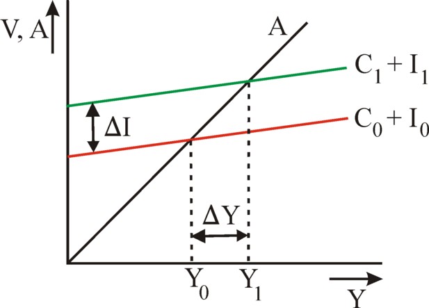
Figure 1: The commodity market on t=0 and 1
In the west the macro-economic theory of J.M. Keynes has opened the door for the development of growth models for a single sector. Keynes himself has mainly studied the conjunctural phenomena. R.F. Harrod was the first to introduce a growth model, and in it he stresses the dynamics. Several years later E. Domar extended the model with elegant mathematical formulas. Nowadays their results are commonly presented as a whole, which is called the growth model of Harrod-Domar.
It is striking that the publications of successful economists are often reinterpreted by their adherents, and thus their tenor changes. This seems to be the case also for Harrod and Domar. An additional problem is that the publications of Harrod and Domar are placed in professional journals, which a small circulation. Moreover your columnist has the impression that the publication of Harrod is difficult to comprehend1. The present column will present the various views, that exist with regard to the model of Harrod-Domar,
Nearly all textbooks about economics present the one-sector models of Domar and Harrod in the form of difference equations. However the differential form yields a clearer and more precise analysis. Since Domar has presented his theory in the differential form, in the present paragraph his line of argument will be followed2. It must be remembered though, that Harrod has been the first to introduce the idea.
Let t be the time variable. Let Y(t) be the national income, which is composed of a wage sum L(t) and a total profit W(t). This income is realized thanks to the socially possible physical production with a size O(t). Suppose that the price level is P(t), then in general one has Y(t) = P(t) × O(t). At least this relation will be employed in the remainder of the column. Of course in practice some wages will be paid, which do not directly correspond to an available product, namely when the product has not yet been finished. On the other hand, unemployment is conceivable, as long as not all production capacity is occupied. Then the income is smaller than is expected on the basis of the potentially possible product O(t).
Let K(t) be the stock of capital goods, that can be put to a productive use. He is also called the stock of the fundamental fund, or simply the factor capital. To be concrete, it concerns here the equipment with a relatively long lifetime (much longer than a single production cycle), such as machines and real estate. The ratio K(t) / Y(t) is called the capital coefficient. He indicates the number of capital units, that is needed in order to produce a unit of the endproduct. He is a technical coefficient, that mirrors the state of the technological progress in the production process. His differential form is
(1) dK/dY(t) = κ(t)
In this column κ is called the marginal capital coefficient. Due to the time-dependent charachter he can differ from the capital coefficient himself. Harrod does not give a name to κ, although in the introduction of his publication he does stress, that he interprets him as an accelerator. Domar uses in his text the inverse of κ, and calls this the potential social average investment productivity.
Suppose that in an infinitesimal time step dt a quantity dK(t) of capital is added to the stock K(t). The ratio dK/dt is called the investments I(t). Thus the stock K(t) can be interpreted as the result of continuous investments. Therefore K(t) is sometimes called the quantity of investment goods. Now from the formula 1 it follows that
(2) dY/dt(t) = I(t) / κ(t)
At least in this type of growth models it is usual to assume that the propensity to save s = S(t) / Y(t) is constant in time. Here S(t) is naturally the total sum of savings, which the households remit from their income Y(t). In a situation of equilibrium the producers invest the whole amount of savings. In other words, one has I(t) = S(t). It follow immediately that
(3) I(t) = s × Y(t)
Substitution of the formula 3 in the formula 2 yields the differential equation for Y(t)
(4) dY/dt(t) = (s / κ(t)) × Y(t)
Suppose that κ is also independent of the time t. Then the solution for the national income is
(5) Y(t) = Y(0) × e(s/κ)×t
The quantity gY(t) = dY/Y(t) is called the growth rate of the national income. According to the formula 5 one has
(6) gY = s / κ
The parameter gY is constant, and thus the economic system grows with the same growth rate for all times. The independency of κ with respect to time implies, that the capital productivity does not change. This suggests that there is no technical progrsess, in spite of the investments I(t). The explanation could be that the investments are unfinished and therefore are not yet productive. In that situation the growth is caused by the occupation of the still idle equipment3.
The formula 5 has consequences for the development of the factor capital. For one can write K(t) = K(0) + ∫0t I(τ) dτ. Apply the formula 2 in combination with the formula 5, then the result is
(7) K(t) = K(0) + κ × Y(0) × egY×t
The formula 7 shows that for a sufficiently large time t the factor capital has the same rate of growth as the national income.
The economic interpretation is that a growing national income Y(t) and a growing physical product O(t) require a corresponding growth of the equipment K(t), at least as long as the technique does not change. Harrod calls this type of growth warranted (satisfactory). Obviously that rate of growth also applies to I(t), because of het definition I(t) = dK/dt. That is to say, Y(t) - and O(t) -, K(t) and I(t) all three grow with one and the same constant growth rate for all times. In short, the mathematical form is
(8) dY / Y = dK / K = gw = s / κ
In a previous column it has already been noted, that gw can not exceed the sum of the growth rates gL + ga. Here gL is the rate of growth of the professional population, and ga is the rate of growth of the efficiency of labour. Harrod calls this upper boundary the natural rate of growth.
The preceding argument is well known and can be found in any decent textbook about macro-economics. Here it is repeated only in order to define the various variables, and it is to be hoped in an undstandable manner. It is less well known that Domar has included a theory of the capacity utilization in his model4. She is sufficiently nice to reproduce here. The reader remembers that O(t) is the potentially possible production. Therefore the utilization u(t) of the equipment (for a constant price level P) is
(9) u(t) = Y(t) / (P × O(t))
The formula 9 expresses that the producers may decide to keep a part of the production capacity idle. Evidently this results in less income for all involved. Then u(t) is smaller than 1 5.
In this case the formula 1 will pertain to O(t) and not to Y(t). In other words, one has dK/dO = κ×P. For this is simply the state of the technique, apart from the operational decisions about the utilization of the capacity. Suppose again that κ is constant. Then the quantities K(t) and O(t) have apparently the same growth behaviour, with as a consequence that they have equal growth rates for sufficiently large times. Then K(t) will become approximately equal to (κ×P) × O(t). Let the growthrate of K(t) be gK. Moreover the investments still satisfy the formula 3. When these insights are applied to the formula 9, then the result is
(10) u = (dK / K) × (κ / s) = gK / gw
The formula 10 shows, that the economic growth gK can evidently be smaller than the warranted growth gw. However the consequence is that some equipment remains idle. The utilization u is independent of time, because gK and gw are both constants. There is permanently the same percentage of capacity in reserve6. This also explains once more, why the growth gw is satisfactory. As soon as the equality gK = gw is realized, all capacity is used. And this is in principle the aim of all producers.
The point of the capacity utilization is important in the theory of Keynes. She argues that an injection of purchasing power leads to economic growth. For the extra income will motivate the producers to use production capacity, which was idle until then. This extra production generates extra income, which is passed on in a process of income multiplication. It is not per se necessary that the injection of purchasing power installs new equipment (although this is naturally desirable).
For the sake of completeness in this paragraph a short description is given about the equilibrium on the commodity market, for the case that the demand depends on income7. This has the additional advantage that quantities are defined, which are needed later in the dynamic model of Harrod. A market is characterized by a demand and a supply, which must be equilibrated.
Suppose that the consumptive demand is given by the relation C(t) = (1-s) × Y(t). Let the producte demand be I(t) = IA (A of autonomous). The reader sees that in this model the investments do not depend on Y(t). Thus the total (aggregated) demand function is8
(11) V(t) = (1 − s) × Y(t) + IA
The figure 1 presents the formula 11 in a graphic manner.
The supply can be determined from the sum of all incomes, so from Y(t) = L(t) + W(t). For this is just the value, which the production process has generated. Thus it is the value of the nett product, which is offered on the market. The supply is
(12) A(t) = Y(t)
Apparently the supply A as a function of Y is simply a straight line through the origin. It is also drawn in the figure 1.
In the equilibrium the equality V=A holds. The figure 1 shows two of those equilibrium incomes. The first one is Y(0), at the time t=0. The second is Y(1), at the time t=1. Since this column is devoted to growth, one has Y(1) > Y(0), and the difference is ΔY = Y(1) − Y(0). The reader sees in the figure 1, that IA at t=1 must be larger than at t=0. When the national income grows, the equilibrium on the commodity market can only be maintained, as long as the equality IA(1) = IA(0) + ΔIA holds. This change of the autonomous demand does not depend on Y, but it does depend on ΔY. To be precise, ΔIA = s × ΔY. The extra investments influence the national income by means of a multiplier9.
This paragraph is based on two sources10. The explanation by Harrod himself is not very clear, and moreover she lacks mathematical formulas. Footnotes will indicate the parts where your columnist can not follow Harrod.
Harrod prefers in his arguments to consider a stepwise growth of the economy. Your columnist follows him in this, among others in order to prevent confusion. However the consequence is that henceforth the formulas 1-8 must be applied in their difference form, instead of the differential version. For Harrod the capacity utilization is simply u=1. Furthermore it is convenient to use in the formalism the growth factor G(t) instead of the growth rate g(t). The growth factor is defined by
(13) G(t) = Y(t) / Y(t-1)
In the formula 13 t counts the successive time intervals. Each time interval has a duration Δt.
The formula 2 changed into
(14) I(t) = κ × ΔY(t)
In the formula 14 the growth of income ΔY(t) equals Y(t) − Y(t-1). The formula 14 must be interpreted in the sense that the investments I(t) are done during the time interval t, which has as its boundaries (t-1) × Δt and t × Δt.
Harrod is aware that a path of warranted growth exists, with the growth rate gw, which is given in the formula 8 (he was even the first person to invent this idea). The corresponding growth factor is Gw = κ / (κ-s) 11. But what will happen, Harrod wonders, when the growth factor G(t) will deviate from the warranted growth factor Gw? At the time t the producers have generated a product with an added value of Y(t). A disturbance will occur as soon as the aggregated demand C(t) + I(t) begins to deviate from Y(t). Then the commodity market is no longer in equilibrium (see the figure 1)12.
For instance it is conceivable that Y(t) < C(t) + I(t). The demand side is apparently prepared to mobilize additional purchasing power, for instance by borrowing. The producers see the unexpectedly large purchasing power, because they can not supply the goods from their own production, and thus they must break into their stocks. They realize that soon their production capacity may be insufficient. They need to invest again for the following production period t+1, and they adapt their growth expectation in upward direction. That is to say, they expect that the growth factor will obey the relation G(t+1) > G(t). They think that G(t) does not equal the warranted growth factor Gw. It seems to them, that the path of warranted growth requires a faster growth. This requires extra investments.
In the same way it may be that Y(t) > C(t) + I(t). Then the demand lags behind the supply. The producers are forced to increase their stocks of goods. Or they must reduce the utilization u of their equipment. In imitation of Domar they will believe that the growth path G(t) lies below Gw. But contrary to the suggestion of Domar in the formula 10, the producers will not be satisfied with this situation. They change to a path of slower growth, and decrease the growth of the investments.

It seems obvious that the producers will adjust the growth factor according to (what else?):
(15) G(t+1) = G(t) × (C(t) + I(t)) / Y(t)
For instance, when the demand has been 5% above their supply, the producers will base their investments on the expectation of a growth factor G(t+1), that is 5% larger. The formula 15 can be rewritten by using C(t) = (1-s) × Y(t) and the formula 14:
(16) G(t+1) = G(t) × (1 − s + κ) − κ
The formula 16 is an inhomogeneous difference equation of the first order. The solution consists of a general part and a particular part13. The particular solution is G(t) = Gw = κ / (κ-s), and the general solution of the homogeneous equation is G(t) = α × (1 − s + κ)t. It desired the reader can check this by substituting them in the formula 16. When this is combined with the initial condition G(0) for G(t) at t=0, then the general solution of the inhomogeneous difference equation becomes
(17) G(t) = Gw + (G(0) − Gw) × (1 − s + κ)t
As is to be expected, the growth is stable for G(t) = Gw. As soon as a deviation occurs, G(t) will move away from Gw with the passage of time14. The figure 2 illustrates this in a graphical manner. The behaviour of the formula 15 may be rational for the individual producer, but it leads to a collective irrationality. When the system grows a bit too fast, the producers will invest more. When the growth is too slow, then they restrict their investments. Therefore Harrod says that the growth behaviour balances on the knive edge.
Harrod himself is not clear about the cause of the economic disturbances. He suggests among others, that G(t) may deviate from Gw as a consequence of seasonal variations, of a changing consumption pattern or of a changing balance of trade. Jan Pen gives in his book Macro-economie a qualitative description of the dynamic equilibrium according to Harrod15. Pen blames the producers for the economic disturbances. Namely, they will sometimes invest too much or too little, with the result that Y does not coincide with C+I. Even the formula 16 seems to blame the investments for the disturbance, because the consumption always obeys the relation C= (1-s) × Y.
Although also Harrod discusses the instabilities on the market, this is not addressed by his formulas. In his argument the producers are simply surprised by the unexpected change in the growth path of the national income. He relates this to a change in the marginal capital coefficient, a find that is ignored by his adherents. This makes the whole theory somewhat confusing, at least for your columnist.
And despite the alarming presence of the knive edge, such as is shown in the figure 2, Harrod is not pessimistic. He writes16: "As actual growth departs upwards or downwards from the warranted level, the warranted level itself moves, and may chase the actual rate in either direction. The maximum rates of advance or recession may be expected to occur at the moment when the chase is succesful". This is not so much a description of an instability, but of an gradual change in the economic variables. Thus the model of Harrod loses much of its dramatic character.
Nevertheless the model of Harrod has given cause for concern. Namely, the factor labour does not appear in it. There is no reason why the warranted growth gw should coincide precisely with the natural growth of the quantity of effective labour hours. Notably a warranted growth could lead to a structural unemployment.
Especially the economists with a neoclassical orientation are unhappy with the find of Harrod. For them the idea of a structurally unstable market economy is a nightmare. Also they do not accept the suggestion that the labour market may be structurally in disequilibrium. Thus the model of Harrod became a stimulus for the development of a neoclassical alternative, notably the model of Solow, which is discussed in a previous column.
To be concrete, the growth model of Solow critisizes the assumption of a constant capital coefficient17. Namely, the formula 12 suggests that the contracting of extra workers will not cause a growth ΔY. And this suggestion is rather strange. For it is possible to make a product in various ways. Up to a certain degree a substitution of the factor capital by the factor labour (and reverse) is possible.
Thus the substitution of the production factors can also mitigate the knive edge instability. For instance, suppose that a situation occurs with Y < C+I. That is to say, there is an excess of demand. Now the producers could in the first instance forgo new investments, and instead they could engage new workers. Thus would reduce the chance that too much capital goods are accumulated. Besides the capital coefficient K/Y is lowered in this way. The level of the warranted growth shifts upward18. In a situation of large unemployment this even becomes likely, because then the wage level is low. It is attractive for the producers to contract more workers.
Apparently the idea of the constant κ is questionable. Now Harrod himself has already pointed this out, so that the criticism of the neoclassical groups is somewhat overdone19. The growth model of Harrod has really its merits, namely that it shows how the economic system can derail in situations, where the alleviation due to the factor substitution is insufficient.
Finally is is interesting to present the interpretations from an unexpected source, namely those of the Leninist economists from the former Soviet Union. One would expect a certain enthusiasm about the find of Harrod, but then one is mistaken. Although his pessimism with respect to the operation of free markets is welcomed, the general comment is that he ignores the economic essence (namely the conflict of interests between the factors capital and labour)20. Since they are fervent adherents of the central plan-economy, they are convinced anyway about the instability of the free market. Besides the plan-economy provides for a complete picture of the social production, so that she can never exhibit a collective irrationality. Therefore the work of Harrod is of little practical interest for these economists, even though they praise his intellectual performance. The studies of Eva Müller, which have been described in previous columns, do not address this type of arguments about the behaviour of producers.