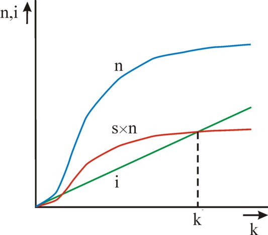
Figure 1: The behaviour of n and i versus k
The American economist R.M. Solow developed in 1956 a growth model, which describes the economic system as a whole, that is to say, as a single sector or branch. The model interprets the national income with the help of a production function, which has the advantage that the factor labour is included explicitely as a variable in the model. Thus the model encompasses the technological progress, in the sense that the labour productivity (ap) can rise. The Solow model in its basic form is quite simple, because it can be formulated in an analytic manner. The seamy side is that in the basic model a number of restrictive assumptions are made. If those are abandoned, then the model has a more universal validity, but the solution can only be obtained by means of numerical methods. The more advanced textbooks about macro-economics usually do give an explanation of the Solow model. Yet it is justified to dedicate a column to the model, since elsewhere the explanation can be incomplete or vague1.
In a previous column the simple national income model is presented, in imitation of the East-German economist Eva Müller. That model starts with the formula N(t) = K(t) / κ(t), where t is the time variable, N the national income, K the factor capital (also called the stock of capital goods, or the stock of fundamental fund, and κ is the capital coefficient (with as its inverse thecapital productivity, or effectivity of the fundamental fund)2. Solow replaces this formula by a more general one, which includes also the factor labour L(t):
(1) N(t) = F(L(t), K(t))
Here the symbol F represents a function, with L and K as her variables. F is called a production function. Often the units of N, L and K remain vague. In this column L will be expressed in the number of working-hours, and N and K in money sums, based upon the national currency. At the end the column will briefly return to this choice.
A striking aspect of the production function is the variety of combinations (L, K) of labour and capital, that lead to the realization of the same national income N. Apparently both production factors can be mutually exchanged. Such a situation is called the substitutionality of the production factors. In other words, the formula 1 represents a multitude of mutually different production techniques. At the time t the producers can make a choice from an infinite number of production techniques.
In the previous column, which has been mentioned before, it turns out that the factor capital K changes with time due to wear and investments. During a time interval Δt the change ΔK(t) = K(t) − K(t-Δt) equals
(2) ΔK(t) = i(t-Δt) − v × K(t-Δt)
In the formula 2 i represents the gross investments, and v×K the discarded equipment. The variable t now refers to a time interval, that is to say, the space of time between (t-1) × Δt and t×Δt. In general v will be more or less a constant in time. The gross investments can be separated in the nett investments iN, and the replacements iV. It is usually assumed, that the replacements compensate for the discarded equipment. Then one has iV = v × K(t-Δt), where v is called the rate of replacement.
The gross investments must be paid from the national income N. In other words, one has
(3) i(t) = s × N(t)
The quantity s is called the propensity to save, or somewhat oldfashioned the rate of accumulation. It is commonly assumed that the propensity to save does not change with time. The formula 3 contains an important assumption. Namely, the producers use the total of the savings balance S=s×N of the households for investments. The savings balance and the investments are in equilibrium according to i(t)=S(t). The households spend the remaining part C of the national income completely on consumptions:
(4) C(t) = N(t) − S(t)
The formulas 1, 2 and 3 can be combined into
(5) ΔK(t) = s × F(L(t-Δt), K(t-Δt)) − v × K(t-Δt)
The formula 5 makes it possible to compute the development of K(t) with time in time steps Δt. Subsequently other quantities can be derived, such as N(t), by means of the formula 3.
In the formula 1 the factor labour L can also vary in size with time. The Solow model distinghuises between two growth processes:
The most important quantity in the growth model of Solow is the capital intensity k(t). She is defined as k(t) = K(t) / L(t). If the capital intensity is constant with time, then there is a direct relation between the factor labour and the factor capital. Then the growth of L, such as in the formula 6, must lead in an automatic manner to a growth of K. According to the formula 2 the investments i(t) must take this into account, In that situation the new added labour will produce under exactly the same conditions as the already present labour.
The core of the growth model is the transformation of the factors labour L(t) and capital K(t) to the capital intensity k(t). This is only possible, when the production fuction has constant returns to scale5. That is to say, if L and K are scaled up with a constant μ, then N will also scale up with the same μ. In mathematics such a function is called homogeneous of the first degree. An example of a production function, which satisfies this demand, is the well-known Cobb-Douglas function
(7) N(L, K) = α × Lβ × K1-β
In the formula 7 α and β are constants, where β is positive and β<1.
The transformation is realized by dividing the left- and right-hand sides of the formula 1 by L. Then the homogeneity, which has just been mentioned, leads to F/L = F(L/L, K/L) = F(1, k). Define n=N/L and F(1, k) = f(k), then the formula 1 changes into
(8) n(t) = f(k(t))
The transformation has eliminated the quantities L and K from the equation, and instead the quantity of capital per effective working-hour appears6. Subsequently some simple calculations can introduce the quantity k(t) in the growth formula 5. The starting point is the relation7
(9) Δk(t) = (ΔK(t) − k(t-Δt) × ΔL(t)) / L(t-Δt)
If the formulas 5 and 6 are substituted into the formuls 9, then the result is
(10) Δk(t) = s × f(k(t-Δt)) − (v + gL + ga) × k(t-Δt)
In this way Solow has succeeded in writing the change of the capital intensity as the difference of two terms. The first term s × f(k) represents the accumulation per effective working-hour, which during a period Δt must be taken grom the national income. The second term (v + gL + ga) × k represents the necessary investments per effective working-hour, which are required for each period. They must compensate for the discarded equipment, for the growth of the population, and for the rising labour productivity.
In the figure 1 the two terms are shown in a graphic manner. Due to the assumed constant rates of growth the second term is simply a straight line. The behaviour of the first term is less self-evident. Here the shape of n(t) and of the accumulation s×n are based on the neoclassical concept of the marginal product8. Strictly speaking that concept has been developed for micro-economics, but Solow uses it in a macro-economic interpretation. That comes about as follows. The number of effective labour-hours in a society is more or less fixed, at least for the medium term. Then for a given state of the technology there is an optimum for the stock K of capital goods, and thus for the capital intensity k. Below that optimum the marginal product ∂n/∂k rises as a function of k, and above the optimum it falls. The reader may recognize both domains in the figure 1. The marginal product is naturally always positive, except in situations with an extreme excess of capital goods. The economic system will commonly reside in the second domain, where the marginal product falls.
The figure 1 shows that in the domain of the falling marginal product two ranges of k can be discerned. These two ranges are separated by the point k=k*. In the first range the accumulation is larger than the necessary investments9. So much capital goods are put into use, that the quantity of capital per effective working-hour actually increases. This simply means, that the capital intensity will increase. In other words, one has Δk > 0, and k(t) shifts to the right along the horizontal axis. In the second range the accumulation is smaller than the necessary investments. Here one has Δk < 0, and k(t) shifts to the left. Therefore in both ranges of k there is the tendency to move k(t) towards the equilibrium point k*.
As soon as the equilibrium point k=k* has been reached, one obtains Δk=0 and the capital intensity will stabilize. The economic system has reached a growth trajectory, where the proportion of L and K remains stable. There is no longer a factor substitution between capital and labour. The formula 9 shows this aspect from a different perspective. If Δk=0, then according to this formula one has
(11) ΔK / K = ΔL / L
The growth rates of the two production factors are identical. Due to the formula 1 and the homogeneity of F the national income N(t) will also grow with the growth rate according to the formula 11. This growth path is called the satisfactory or warranted growth, and the corresponding growth rate is indicated by gw. In general ΔL/L will determine the size of gw. For the growth of the population and the progress are externally given. The capital growth and the economic growth must adapt to them. As a consequence one has
(12) gw = gL + ga
This argument has in essence completed to find of Solow.
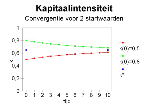
In conclusion this paragraph will illustrate the model with an example. Suppose that the national income is given by the formula 7, with α=1 and β=0.67. Then it follows that n(k) = k0.33. Let the propensity to save be equal to 0.15. Assume moreover that v + gL + ga = 0.2. Then the formula 10 can be used to calculate the equilibrium value of k, with the result k*=0.65. Suppose now that two kinds of this society exist, with however different initial values k(0) = 0.5 and 0.8. The figure 2 shows, how the growth trajectories of these two societies will converge in time. Note that due to the formula 12 the warranted growth rate is not yet known. This requires a knowledge of the value of v.
In the preceding columns it has been stressed that economists are interested mainly in the size of the consumption. In the optimal growth path the consumption will be maximal. The economist E.S. Phelps has shown, how the model of Solow can be used in order to find the optimal growth path. He has derived the condition, that the capital intensity must satisfy, and he has called her the Golden Rule10. The households are able to steer the economy to the optimal point, since they determine the value of the propensity to save s.
The starting point is the formula 4. It the left- and right-hand side are divided by L, then one finds C/L = n − S/L = f(k) − i/L = f(k) − (v + gL + ga) × k. Obviously the optimization must lead to the equilibrium point k=k*, because this is the inevitable end-state of the economic system. Then the optimization condition is ∂(C/L)/∂k* = 0. In other words,
(13) ∂f(k*)/∂k* = v + gL + ga
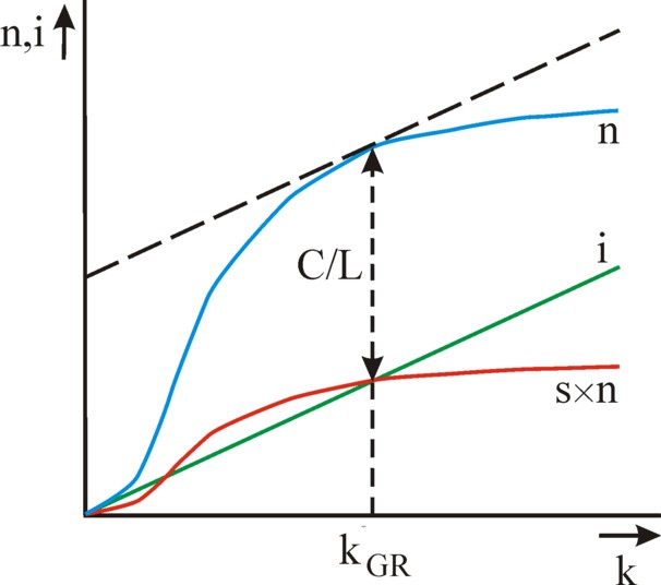
The formula 13 is the Golden Rule. The solution of the Golden Rule is the point k* = k*GR, which is called the Golden Rule level of capital. The Golden Rule guarantees that the highest level of consumption is reached. The figure 3 illustrates the Golden Rule in a graphical manner. The Golden Rule level of capital k*GR is the point, where the tangent to the curve n=f(k) has the slop v + gL + ga. In that point the consumption per effective working-hour equals f(k*GR) − (v + gL + ga) × k*GR.
The propensity to save sGR, which yields the Golden Rule level of capital, is a compromise between the ambition to, on the one hand, enlarge the national income n(k*) by means of investments, and to, on the other hand, protect the consumption n-i against the desire to invest. In other words, it must be avoided that the consumer goods become scarce due to claims on the national product for the replacement of discarded capital goods and for the supply of capital to the extra labour. A concrete example of a faulty allocation is the building of expensive and maintainance-prone business premises.
The reader can compare the figure 2 with the figure 1, and then sees that the households must diminish their efforts to save in order to reach the point k*GR, starting from the figure 1. For the curve s×n drops down. They will be glad to do this, since a smaller s increases immediately the consumption C/L. However, this aspect shows that the change of the propensity to save causes a temporary instability. The system will gradually adapt to the new situation. It would be painful, if there was the need to raise the propensity to save. In the first instance more savings imply a falling consumption. The consumption will exceed her original value only after a sufficient rise of the stock of capital goods and of the national income.
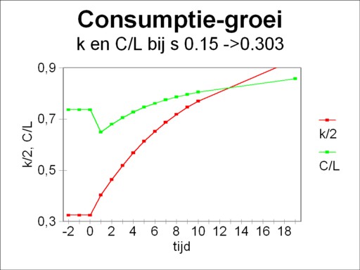
Perhaps an example will clarify this aspect. Take again the data of the example in the preceding paragraph. According to the formula 13 here one has k*GR=1.865. Since the economic system has converged towards k*=0.65, more savings are needed, and thus the propensity to save of s=0.15 does not suffice. The application of the formula 10, with Δk=0 and k*GR=1.865, yields a new propensity to save of sGR=0.303. Suppose that the new savings regime starts at t=0, then the figure 4 shows the development of the consumption C/L with time. For the sake of completeness also k(t) is shown (scaled down to 50% for reasons of presentation).
The loyal reader of this portal will not be surprised by the Golden Rule. In for instance the column about the one-sector models of Eva Müller the figure 2 shows how the propensity to save can be chosen in a deliberate attempt to reach tot maximal consumption.
The criticism is directed towards the neoclassical assumptions, that underlie the growth model of Solow. Firstly, production functions with a homogeneity of the first degree, such as the Cobb-Douglas function (formula 7), are not particularly suited for the description of the economic reality. That is caused by their hallmark of constant returns to scale. For enterprises can usually realize efficiency gains, when they increase the size of their production process.
A second point of concern is the aggregated capital K as a variable in the macro-economic production function, such as the one in the formula 1. Unfortunately an aggregation of capital goods is only possible by making use of their prices. And those prices depend on the distribution of the national income over the wages and the profits. If the distribution (allocation) is changed, then the production function will obtain a completely different form. That is to say, when in a production function the variables are replaced by price sums, then she is actually no longer a production function. The intertwined technology of the various production factors is eliminated.
Yet another point of criticism is the neoclassical assumption that markets can be cleared completely. Thus Solow supposes in his model that the employment is complete, and that the savings and investments are in equilibrium (I=S). These assumptions have been undermined by the theory of Keynes. The investments I can actually fall below the savings S. This will lead to a shrinking national income N 11.