One-sector growth models with production functions

First insertion on Heterodox Gazette Sam de Wolff: 2 april 2014

Now that a previous column has succinctly explained production functions, the present column will present several macro-economic growth models from the book Mathematical models of economic growth¹ of the well-known Dutch economist Jan Tinbergen. A relation will be derived between the growth rates of the economic variables (capital, labour, technical development). The starting point is the Cobb-Douglas production function. The situation with complementary factors is also studied.

In the mentioned column it is stressed, that production functions contribute little to the theoretical insight at the macro level of the economy. The arguments in the present column are outdated from a scientific perspective, and are merely important for historical reasons. It would be unfair to reproach Tinbergen with his theoretical error. Its undermining, notably the theory of Sraffa, was not published until 1960, two years before the publication of Mathematical models of economic growth. In 1962 the theory of Sraffa was still controversial. For instance, between 1962 and 1966 the famous North-American economist Paul Samuelson tried in various ways to refute the theory. He did not succeed².

It is understandable that Tinbergen retains the then common economic growth models, which have been developed, among others, by the English economist Roy Harrod. Then Tinbergen already specializes in the analysis and development of methods and instruments for economic planning. His interest concerns mainly the practical applications and the policy formulation. The models in the present column are limited to an economic system with one productive sector, however with various scarce production factors. Therefore they offer more flexibility than the one-sector models, which have been presented in a previous column, and merely follow the development of the factor capital.

Model with perfect substitution of production factors

The models of Tinbergen use merely two production factors, namely the capital K and the labour L. Besides they take into account the technical progress, which advances with time. Tinbergen wonders how these factors affect the growth of the domestic product Y ³. Then the choice for the popular Cobb-Douglas function is obvious⁴

(1)     Y(t) = A(t) × L^λ × K^μ

In the formula 1 the term A(t) takes into account the technical progress. It is sometimes called the total factor productivity. The parameters λ and μ are constants. The same gross product can be generated with various quantities of capital, due to the substitution of K and L. In this model the capital coefficient κ = K/Y is variable, contrary to the Harrod-Domar models. That is a crucial difference. In fact the presented model is similar to the growth model of Solow. Solow uses a linear-homogeneous production function, which is somewhat more general than the Cobb-Douglas function.

Cobb-Douglas production functions have the special property, that they can describe both the Hicks- and Harrod-neutral progress. The form in the formula 1 is Hicks neutral. However, it can be rewritten as Y = (A^1/λ × L)^λ × K^μ, and that form is precisely Harrod-neutral. Often A(0)=1 is assumed. Tinbergen prefers A(t) = (1 + g_A)^t, where g_A is a constant. Note that for this case the growth rate (∂A/∂t) / A is apparently equal to the natural logarithm ln(1 + g_A). Therefore, for a sufficiently small value of g_A this quantity approximates the growth rate of A.

In the present paragraph it is assumed that μ = 1 − λ. Then the production function is linear homogeneous, and the productivity does not depend on the chosen scale. It is true that Tinbergen recognizes that the separate enterprises commonly profit from an increased scale, but he assumes that this effect is cancelled at the level of the national economic system as a whole. Next the factor prices are equated to the marginal productivities, that is to say, p_L = ∂Y/∂L en p_K = ∂Y/∂K. The loyal reader knows from the mentioned column, that this assumption is actually faulty, since here Y and K are aggregated quantities. It can naturally simply be assumed, that these relations still hold (for what it is worth)⁵.

Figure 1: Supply curve of labour

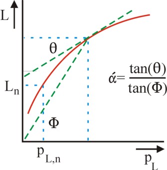
Let the normal price of labour be p_L,n, and suppose that then the professional population has a size L_n. When the price changes to another value p_L, then the willingness to work will change accordingly. Suppose that this behaviour obeys the formula

(2)     L = L_n × (p_L / p_L,n)^α

In the formula 2 α is a constant, which is called the elasticity of the labour supply. The figure 1 is a graphical presentation of the formula 2. Apparently one has α = tan(θ) / tan(Φ), where θ is the slope of the supply-curve of the factor labour, and Φ is the slope of the line through the point (p_L, L) and the origin.

In the figure the elasticity α has a positive value, but she can be negative as well. In that case the labour supply decreases, according as p_L (the wage level) rises. In that sense the supply curve of labour is no more self-evident than the demand curve of labour. In an identical manner a formula can be stated for the factor capital:

(3)     K = K_n × (p_K / p_K,n)^β

The option of the elastic supply adds an element, which is missing in the model of Solow. A special case of the formulas 2 and 3 occurs, when the supply elasticities α and β are zero. Namely, then the supply of K and L will always be equal to K_n and L_n, the quantities which belong to the normal factor prices. The corresponding supply curve in the figure 1 is a horizontal line. This assumption of a completely inelastic supply will be made in the present model, at least for the moment. Then one finds for K the usual relation

(4)     ∂K_n / ∂t = σ × Y

Here σ is the constant savings rate. The formula is based on the assumption, that all savings are invested.

The formula 4 shows, that the factor capital grows with time. That growth is caused partly by the natural population growth:

(5)     L_n(t) = L_n(0) × (1 + g_L)^t

In the formula 5 g_L is apparently approximately equal to the growth rate of L_n. Moreover, the normal price of the factor labour can increase, because due to A(t) the number of effective labour-hours increases. That will increase the productivity per worker. This development leads to

(6)     p_L,n(t) = p_L,n(0) × (1 + g_p,L)^t

However, since this model assumes a completely inelastic supply, at least for the moment, the formula 6 is superfluous. Tinbergen even believes, that the supply of capital will always be completely inelastic (β=0), so that the formula 3 can be ignored again⁶.

Now all formulas are available for the calculation of the relations between the various growth rares. The formula 1 can be inserted into the formula 4, using the formula 5. Thus one finds a first order differential equation in K_n(t), which can be solved in a straightforward manner⁷. The result is the solution

(7)     K_n^λ = K_n(0)^λ + λ×σ × L_n(0)^λ × { ((1 + g_A) × (1 + g_L)^λ)^t − 1 } / (g_A + λ×g_L)

Tinbergen justly states, that this behaviour of K is less simple than the common statistical methods suggest. It is striking that the initial state at t=0 determines the later development. The formula 7 yields an important building stone for the analysis of the relation between the growth rates.

A popular trick is to rewrite the growth rate as g_Y = (∂Y/∂t) / Y = ∂(ln(Y)) / ∂t, where ln() is the natural logarithm function. Apply this trick to the Cobb-Douglas function in the formula 1, then one finds

(8)     g_Y = ln(1 + g_A) + λ × ln(1 + g_L) + (1 − λ) × (∂K_n / ∂t) / K_n

If desired, the first two terms can be rewritten by means of the approximation ln(1 + x) = x + O(x²), at least for small growth rates. The last term in the right-hand part of the formula 8 is simply the growth rate of capital g_K.

Since g_K varies with time, g_Y is also a functiom of t. For t=0 the formula 8 takes on the form g_Y(0) = g_A+ λ×g_L + (1 − λ) × σ × (L_n(0) / K_n(0))^λ. It is also possible to combine the formulas 1 (still with μ = 1-λ) and 7 in order to calculate the behaviour of the capital coefficient κ=K/Y. Note that for large values of t K_n^λ approaches λ×σ×A × L_n^λ / (g_A + λ×g_L). Therefore in the limit of t→∞ one has

(9)     κ = λ × σ / (g_A + λ×g_L)

Apparently in the long rung the capital coefficient does become a constant. Note that in the absence of technical progress (that is to say, for A=1) the formula 9 reduces to the Harrod-Domar relation κ = σ / g_w. This completes the foundation of the growth model of Tinbergen. On p.36 of Mathematical models of economic growth it is also shown, that the growth rates of K, L and Y can be calculated even for the case, when the labour supply is not perfectly elastic. A table gives the growth rates in situations, where λ=¾ and the elasticity has values of α = -1, 2 and infinity. In those cases the growth rate g_p,L of the normal price p_L,n of labour from the formula 6 also emerges in the table. She affects the other growth rates.

Evaluation of the model

In the preceding paragraph the growth model of Solow, which has already been published in 1956, has been mentioned several times. Indeed the question arises, what the model of Tinbergen adds to that model. According to the model of Solow a warranted growth occurs, as soon as g_Y = g_K = g_A + g_L is satisfied. The first identity returns in the described model, where according to the formula 9 Y and K are proportional. Next the second identity can be derived from the formula 8, at least in the form

(10)     g_Y = (g_A / λ) + g_L

Figure 2: Tinbergen in 1965

In the growth model of Solow the factor λ does not appear, because he employs a production function of the form λ Y = F(K, A(t) × L). Tinbergen has placed A(t) before the F- function. Furthermore, Tinbergen calculates the time behaviour of the system by means of the formula 7. Solow prefers to express the formulas in terms of the capital intensity k = K / (A×L), and then shows that the system will move towards a state with a constant k.

Furthermore, Solow advances a step further than Tinbergen, because he analyzes a state, where the consumption per worker will be maximal. From this situation he derives his Golden Rule of capital, which dictates the optimal savings rate σ. Tinbergen omits this approach, perhaps because he does not trust her. His argument is explained in a previous column. In short, the policy maker would be obliged to maximize both the present consumption and the consumption of future generations. Here he would have to weigh the interests of succeeding generations.

And finally Tinbergen attaches value to the presence of the elasticity α of the labour supply in the model. For, besides the optimal consumption the maintainance of the full employment is also one of the policy goals. The policy makers can steer the employment by restricting the wage development p_L,n. When α is positive, then according to the model the growth of the wage will inhibit the production and the employment. Tinbergen illustrates this by means of the mentioned table, with values of α between 2 and infinity. On the other hand, when αis negative (α=-1 in the table), then the wage rise turns out to stimulate the economy.

The book does not explain the calculations of the quantities in the table. It is clear that the formula 6 predicts a rising p_L,n. Thus in the formula 2 the value of p_L/p_L,n will fall, which may decrease or increase the quantity L, depending on the sign of α. Note that here L_n will obey the formula 5. Besides, according to the model more savings almost always further the growth. Considering the theories of Sraffa and Keynes these policy recommendations must of course be used with care!⁸

Forms of technological progress

Following Solow, Tinbergen points out, that the labour productivity is given by ap = Y/L = A × (K / L)^1-λ = A × k^1-λ. She increases according as the capital intensity rises, at least as long as λ<1, which is the normal situation. In case of a rising k and constant factor prices p_K and p_L the model makes the surprising prediction, that the share of capital in the national income will rise. See also the footnotes.

Another form of technological progress occurs, when the exponent λ of the Cobb-Douglas function will change. One has λ = (∂Y/∂L) / (Y/L). Since the presented model assumes that p_L = ∂Y/∂L, apparently one has L×p_L = λ×Y. In other words, the share of the factor labour in the national income will fall, when the technological changes lead to a lower value of λ.

The exponent lambda; is sometimes called the production elasticity of the factor labour. It is desirable, that the change in λ will lead to a larger national product Y. Suppose that the change in λ is dλ, then Y will change with a multiplication factor (L/K)^dλ = 1/k^dλ. Apparently, for a positive dλ one wants k<1, and for a negative dλ one wants k>1. In a table Tinbergen gives the development of the growth rates for the case λ(t) = λ(0) + Λ×t, where Λ = dλ/dt is a constant⁹. There is more latitude, when the requirement μ = 1 − λ is abandoned. According to Tinbergen the statistical data show, that for a long time λ has hardly changed, which has the consequence, that the distribution of the national income between the factors capital and labour has also been stable.

Models with complementary production factors

Finally p.45 and further in Mathematical models of economic growth briefly describe the situation, where no substitution of production factors occurs. In that case there is no continuous production function, but merely a discrete number of production techniques. In a previous column this is called a production process with complementary factors. Incidentally, this situation does not occur frequently. An example is the weaving of cotton in India, half a century ago, which was done both at home on simple weaving-looms and by means of machines¹⁰.

Suppose two techniques are available, numbered 1 and 2. Suppose that the technique 2 is most capital-intensive, so that one has k₂ > k₁. Suppose that the professional population has a size L_n, and the capital stock is K_n. Finally, suppose that one has K_n / L_n < k₁. In this situation there is an excess of labour, so that in principle the wage level can become arbitrary low (the "reserve army of unemployed"). A minimum wage p_L,n must be introduced in order to prevent the starvation of the workers.

A sound policy will take care that the capital stock K_n increases faster than the population. At a certain time the relation K_n / L_n = k₁ will hold, so that all available labour is employed. Now the wage level is no longer zero, but indeterminate. When K_n grows even further, the technique 1 will no longer be satisfactory, because she would leave some capital unemployed. The socially applied production technique becomes a mixture of the techniques 1 and 2. In fact during this phase the substitution of production factors is possible. The reader can find a careful analysis of this phenomenon in the column about the substitution of the means of production in the theory of Sraffa, a five-finger exercise of your columnist. In another column the same phenomenon is explained by means of the theory of algebraic sets.

In this phase of substitution isoquants can be drawn. In fact these are the curves of technological possibilities. Tinbergen states, that in this situation both techniques will evidently pay the same price p_K,n for capital, and for p_L,n as well. Assuming that one has p_K,n = (Y − p_L,n×L) / K for both techniques, one can calculate in a straightforward manner that

(11)     p_L,n = (k₂×ap₁ − k₁×ap₂) / (k₂ − k₁)

In the formula 11 ap_i is the labour productivity of the technique i. Apparently, now the wage level is fixed.

According as the stock of capital K_n keeps growing, more of the technique 2 must be applied, at least as long as full employment is desired. Finally, K_n will have grown so much, that even the technique 2 can no longer absorb all capital. Here the situation occurs, where the market price p_K,n will become arbitrary low. This phenomenon is not purely fictitious, because both Karl Marx and John M. Keynes predict the fall of the interest rate in the long run.

1. See chapter 3 in Mathematical models of economic growth (1962, McGraw-Hill Book Company, Inc.) by J. Tinbergen and H.C. Bos. (back)
2. By now, the loyal readers of this portal know that economics in the twentieth century has been dominated by the ideological struggle between the western and Leninist economists. Therefore, one would expect, that the Leninist economists are avid adherents of the theory of Sraffa. In reality, they have reservations. A typical example is the book Von Keynes zur neoklassischen Synthese (1976, Verlag Die Wirtschaft) by the Russian economist I.M. Osadchaia. The Russian edition dates from a few years before, but amply before the establishment of the theory of Sraffa. Indeed Osadchaia admits on p.126: "Many economists believe, that the criticism of the homogeneity of capital is decisive for the refutation of the marginalistic (E.B.: neoclassical) theory. ... With regard to the crisis of the marginalistic theory of distribution this criticism is meaningful, because she proves the decay and the crisis of the doctrine, which in the bourgeois political economics has dominated for almost a century". So far, so good. But thirty pages before he discusses the Cobb-Douglas function, and the factor substitution as well. On p.93 he argues: "It is obvious that there is a dependency between the movement of the real prices of the production factors and their use in the production. A rise of the wage level stimulates the substitution of the living labour by the fixed labour (EB: capital goods). Often it depends on the wage level, whether more or less capital intensive production methods are chosen". This is highly remarkable! For the essence of the theory of Sraffa is, that the choice of the technique is not clearly correlated with the development of the prices of the production factors. (back)
3. See p.32 in Mathematical models of economic growth. Tinbergen does not explain how the domestic product differs from the national income. It is common to include in the national income also those earnings, that are generated with the domestic production factors abroad. Since the presented model does not consider foreign states, the domestic product and the national income apparently coincide. (back)
4. The reader is reminded, that an explanation of production factors in general, and of the Cobb-Dougles production functions in particular, the mentioned introductory column can be consulted. This is even recommended for a good understanding of the present column. (back)
5. Then the neutral character can be studied in depth. The profit share of the national income is K×p_K, and the wage share is L×p_L. In the Hicks neutral situation these are respectively K×A × ∂F/∂K and L×A × ∂F/∂L. The ratio of the profit part and the wage part is k × (∂F/∂K) / (∂F/∂L). For a linear-homogeneous function one has F(K, L) = L × F(k, 1) = L × F(k). So ∂F/∂K = ∂F/∂k and ∂F/∂L = F(k) + k × ∂F/∂k. Apparently the ratio of the profit part and the wage part merely depend on k. Therefore a constant capital intensity will guarantee, that the rentiers and the workers each keep their share in the national income. That defines the Hicks neutral state.
   In the Harrod neutral situation the same rule holds, but now one has F(A×L, K) = L × F(A, k) = L × F_A(k). In both cases κ = K/Y is a function of only k. Therefore, a constant capital intensity implies naturally a constant capital coefficient, for linear-homogeneous production functions. (back)
6. See p.34 in Mathematical models of economic growth. (back)
7. The differential equation is ∂K/∂t = σ × (1 + g_A)^t × L(0)^λ × (1 + g_L)^λ×t × K^1-λ. Define for ths sake of convenience ζ = σ × L(0)^λ and η = (1 + g_A) × (1 + g_L)^λ. Then one has K^λ-1 × dK = ζ × η^t × dt. The soultion is K^λ = constant + λ×ζ × e^{t × ln(η)} / ln(η). At t=0 one finds for the integration constant the value K(0)^λ − λ×ζ / ln(η). The result is K^λ = K(0)^λ + λ×ζ × (η^t − 1) / ln(η). Apply for the sake of convenience for a small value of x the approximation ln(1 + x) = x, then finally one has K^λ = K(0)^λ + λ×ζ × (η^t − 1) / (g_A + λ×g_L), which was to be proven. (back)
8. In Winterrozen voor een kwakzalver the Flemish writer Johan Daisne parodies the scientific progress (p.24): In his dream he suddenly got the insight and the recognition that father, the ridiculous charlatan, the mad boniseur, the frantic preacher of a "paradigm" without end or sense, of "ideas" which cohered like dry sand, nevertheless, and precisely because of this, had been his predecessor, his immediate, valuable, yes even indispensable guide. It is true that the negative example of father had scared him to such an extent, that he, warned, always and everywhere had done exactly the opposite of what the wretched autodidact had once proclaimed or done. Until now suddenly, after half a life of incredible blindness, it became clear that this "opposite" was merely a correction of procedure, a mise au point of method. The negative example of the would-be scientist had indeed, as an example, created a reverse archetype, built with all the faults and impurities of its primitive apparatus, but it had nevertheless been a remarkable and indispensable piece, after which he, as the true scientist, had been able to come and make the sound positive of it. (back)
9. See p.39 in Mathematical models of economic growth. (back)
10. On a smaller scale this phenomenon is also observed in the Netherlands. Thus in Mensen zonder geld by Jan Mens it can be read: Not a single dime can be earned, all comes cheap from elsewhere and the large furniture factories fire their workers. For a dime they fill your house with furniture, but do not ask what that junk looks like! In former days, yes, then the profession was still worthwhile. You did make long working-days, but when you produced such a fine, bowed pier-table, or a bulky walnut chiffonière, well, that gave at least satisfaction. Look at the products now: everything is straight; you may as well place a few orange cases in your room. And now they even introduce steel furniture! Oh Lord, that is completely crazy, so to say. Steel furniture, who has ever heard that on the violin? Where will the good old profession end? (back)