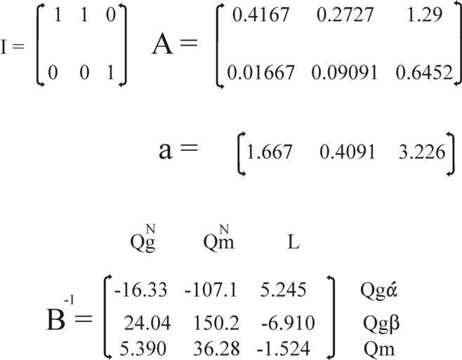
Figure 1: matrices I, A and B-1, and the vector a
In a previous column it has been explained how the formation of prices is realized in the various economic paradigms. The present column is a direct continuation of that text. In an example it will be shown how the substitution of the production factors relates to the change of the production technique. The example uses the neoricardian model of Piero Sraffa. An attempt is made to connect this formalism to the neoclassical substitution of production factors.
The reader will not find the contents of this column in the introductory text books about the neoricardian paradigm1. In fact it is little more than a five-finger exercise, which is an obligatory occupation for any researcher, and which in case of the theory of Sraffa yields such rewarding results2. So although one must not expect pioneering results in this column, it is all still sufficiently interesting to publish in the Gazette.
In order to restrict the length of the text, the mathematical and economical explanation of the model will be omitted. The reader can find her in the preceding column, just mentioned. For the sake of convenience the example is again the familiar economic system with two branches: the agriculture and the industry. The agriculture produces corn (with the bale as its unit) and the industry produces metal (with the ton as its unit). Since the theme consists of the switching of the technique, the system must allow for two techniques. Here they are indicated by α and β.
The difference of the two techniques concerns the production methods in the agriculture. In the technique α the agriculture employs the production method τ(g1) and in the technique β the production method τ(g2). In both cases the production method in the industry, called τ(m1), is identical. The technical coefficients for the three methods are summarized in the table 1. The reader can also find this table in the column about the choice of the technique in the neoricardian paradigm. Henceforth the text will regularly revert to the results of that column.
| agriculture | industry | ||
|---|---|---|---|
| τ(g1) | τ(g2) | τ(m1) | |
| agj | 0.4167 | 0.2727 | 1.290 |
| amj | 0.01667 | 0.09091 | 0.6452 |
| aj | 1.667 | 0.4091 | 3.226 |
In order to understand the arguments it is essential to study the properties of the two methods τ(g1) and τ(g2). The table 2 displays the differences. The method τ(g1) uses per produced bale of corn more corn and less metal than the method τ(g2). It will be shown that for normal prices the method τ(g2) requires more capital goods than the method τ(g1). The cause is the high price pm of metal in comparison with the price pg of corn.
Furthermore, it is striking that the production of a bale of corn by means of the method τ(g1) requires more labour than for the case of τ(g2). The two numbers refer to the total quantity of produced corn Qg. But it will be shown that the difference also holds for the nett product QgN. The nett product is the commonly used measure for the labour productivity. Therefore in the table 2 the labour productivity of the method τ(g2) is larger than the one of τ(g1).
| hallmark | τ(g1) | τ(g2) | hallmark | τ(g1) | τ(g2) | |
|---|---|---|---|---|---|---|
| corn | much | little | labour | much | little | |
| metal | little | much | nett productivity | low | high | |
| total capital | little | much |
In the column about price formation the fundamental equations for the production in the neoricardian model are given by the formulas 1 and 3. They are repeated here, without the accessory discussion about their meaning:
(1a) QN = (I − A) · Q
(1b) L = a · Q
For a start the set 1a-b will be explained as if for each time only one technique is available. In other words, the set refers to either the technique α (with 2×2 matrix Aα and vertical 1×2 vector aα), or the technique β (with ditto matrix Aβ and horizontal vector aβ), but not with a combination of both. The system allows for some dynamics, because the production technique can possibly be changed. That choice would change the productive structure and the corresponding quantities of the production factors. Note however: here and incidentally in the whole column a continuous growth or decrease of the system will not be considered.
Suppose that each of the techniques α and β must produce the same nett product QN, for instance QN = [3, 0.9]. Calculations show that the technique α requires 30 workers (as representatives of a unit of labour), and the technique β only 27.7. In other words, as soon as the technique α is replaced by the technique β, for instance because the corn has become expensive, then the producer must without delay lay off 2.28 workers3. So there is no gradual substitution of production factors, such as in the neoclassical paradigm. The technological changes are productive shocks. That is also apparent from the needed means of production. For the nett product, just mentioned, the technique α requires Q = [12, 3.1], and the technique β requires [15.8, 6.6]. So the change to β requires an ample doubling of the quantity of metal.
An interesting property of intertwined matrices is that it is unproblematic to display different techniques within a single matrix. Then the techniques coexist within the system, and can be used side by side. In the remainder of this column that representation will indeed be employed. This requires a concession, namely the transformation of the square matrices I and A into rectangular ones with dimensions 2×3. Now the vector a has the dimension 1×3. Both I, A and a are displayed in the figure 1. When subsequently the vector a is pasted underneath the matrix (I − A), then a 3×3 matrix is formed, which will be designated as B.
So henceforth in the formula 1a the matrices I and A will connect the plane (Qg, Qm) and the space (Qgα, Qgβ, Qm). Here Qgα and Qgβ represent the quantities of corn, that at a certain time are produced with respectively the technique α and β. The corn is identical in both cases, and only its production process differs. One has for the total produced quantity of corn the relation Qg = Qgα + Qgβ. And the formula 1b is now an inner product between two vectors with each three elements. Incidentally, for the loyal reader this approach is not new, because it has already been applied in the column about the intertwined matrix for multi period optimization. However, there it is the industry, which can choose between two production methods, instead of the agriculture, like in the present case.
An important observation is that the set 1a-b can simply be rewritten into
(2) Q = B-1 · H
In the formula 2 B-1 represents the inverse matrix of B. The vertical 3×1 vector H has QN as its upmost elements and L as its lowest. That is to say, H = [QgN, QmN, L]. In this case the labour L is distributed over the branch industry and the branch agriculture, and within the agriculture over both production methods. When QN and L are given, then all quantities Q can be calculated simply with the formula 2. So it is an extremely powerful formula.
The formula 2 allows to change the quantity of labour L in a continuous manner. The productive shocks have been eliminated. The reason is evidently, that now the production is a mixture of α and β. This has the consequence, that L is necessarily located between 27.72 and 30. For other values of L negative values will occur in Q, which is not reconcilable with economics. In the same way Qg and Qm remain constrained by minimal and maximal boundaries.
The relation between the vectors H and Q = [Qgα, Qgβ, Qm] has an intuitive logic. For instance, when the nett product is fixed, and society wants to increase L, then this can only be achieved by extending the use of the technique α. For α has a low productivity, and requires a relatively large amount of labour. The immediate consequence is that Qgα must grow, and Qgβ must shrink. In a similar manner the effect on Q of all kinds of changes in H can be studied.
So the matrix B-1 is extremely interesting, and it is displayed in the figure 1. In fact its elements are substitution coefficients. In the figure 1 this is emphasized by displaying above the matrix B-1 the quantities, that can be varied if desired (in other words, the vector H)4. Behind the matrix the quantities are displayed, that are influenced by the corresponding changes. The variation of a quantity in H causes shifts in the sizes (substitutions) of the elements of the production vector Q.
For instance, B-111 = -16.33 indicates, that the addition of an extra unit QgN will decrease the quantity Qgα by 16.33. For according as the product grows for a fixed L, the labour productivity must increase. Then more use must be made of the technique β, so that Qgα decreases. In the same manner for instance B-131 = 5.390 can be explained. A rising nett product for a fixed L requires more technique β, and thus more metal (Qm) as a means of production. An extra bale of corn in the nett product requires an expansion of the volume of metal with 5.390 tons. Etcetera.
The mixing of production techniques, such as is assumed in the formula 2, is surprising. For in the column about the choice of the production technique it has been stated, that always one particular technique will yield the highest capital efficiency. The choice of the technique α or β depends on the wage level. Indeed a mixture of both techniques must result in a suboptimal capital efficiency. The producers have no incentive to maintain such a situation. In fact the formula 2 describes a transitional situation, where one technique in the system is gradually replaced by another one.
But although the logic of economics dictates that the situation with a mixture is not stable, yet she reminds of the neoclassical paradigm. For the nett product QN represents the effective demand for products, and L is the demand on the labour market. A change in the market demand or in the demand for labour leads to an adaptation of the quantities of the production factors, according to the formula 2. However, contrary to the neoclassical belief the adaption lacks any logic. She is determined completely by the available production techniques.
The suboptimal character of the mixture becomes clear, when the system of product prices is considered5. For a detailed explanation of the price theory the reader is again referred to the column about the choice of technique. Also in the present situation with two simultaneous techniques the formulas of the theory can be applied in the usual manner, namely by defining the matrix A as the weighed sum of the separate techniques. The formula is:
(3) aij = f × aijα + (1 − f) × aijβ
In the formula 3 f is the fraction of the labour L, that works with the technique α6. That is to say, 0 ≤ f ≤ 1.
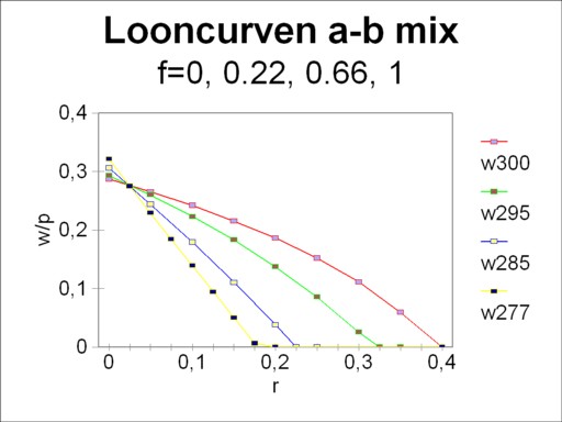
Consider for instance four different mixtures of the techniques α and β, with f=1, f=0.66, f=0.22 and f=0. Suppose that the society wants under all circumstances to produce the existing nett product. When in the mixture f=1, with only the technique α, L=30 workers are employed, then for the other mixtures one has respectively L=29.5, 28.5 and 27.72. The last mixture, with f=0, is purely the technique β. One can think of a shrinking population, which is forced to transform its technique α to the more productive technique β. The figure 2 shows for these mixtures the corresponding wage curves7.
It is immediately clear from the figure 2, that the mixtures f=1 (technique α) and f=0 (technique β) form the technology frontier. The other mixtures lie below this envelope. Only at the switching point of α and β (namely for r=0.024) all mixtures are on the technology frontier. There for a given wage level w/pg all techniques yield the same capital efficiency. The switching point is the pivot, as it were, that rotates the wage curve, according as f (and thus L) changes.
Two mutually opposing economic effects cause the tilting of the curve around r=0.024. On the one hand, the table 1 shows that the technique β has the highest productivity, so that she can guarantee for r=0 the highest wage level. On the other hand, this same table shows that the technique β requires a relatively large quantity of the means of production, so that a lot of interest must be paid. The remittance of interest (in the sense of a rent for the means of production) must be paid from the created nett product. According as the desired capital efficiency increases, the technique β will soon fail to provide for that interest.
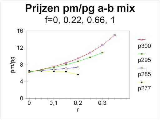
At least as important for this column are the curves of the price ratio pm/pg as a function of the capital efficiency. For in the neoclassical paradigm the prices of the products equal their marginal utility. Their ratio indicates the value, that the society attaches to these products. Each mixture of α and β has her own price behaviour. The figure 3 illustrates that behaviour for f=1, 0.66, 0.22 and 08. Also for these curves r=0.024 is the pivot point. Apparently in general the valuation for metal increases for a rising capital efficiency. Only when tne technique β obtains a preponderant preference, the reverse behaviour occurs. Furthermore, note that in the figure the price ratio is never less than 6.34, namely with the technique β at r=0.178.
The figures 2 and 3 illustrate the balancing influence of the market. The techniques α and β come with their own price systems. However, as soon as they occur in a mixture, the market imposes a uniform price of the labour factors and of the end products. Nevertheless, the prices remain in a perpetual movement, as long as the mixture of techniques changes, for instance during a falling employment L. In the next paragraph the economic tendencies will again be discussed.
Several previous columns pay attention to optimization methods as a means for chosing the best mixture of techniques. In the capitalist system with its private production the application of optimization is mainly limited to the micro level, in the enterprises. But in the former Leninist planning economies this approach was also popular for macro-economic applications.
For the sake of completeness here the optimization problem is formulated again, though it has already been discussed in the related column about price formation. The solution employs linear programming (LP). The LP problem is expressed as:
(4a) maximaliseer Z = p · (I − A) · Q onder de voorwaarden
(4b) (I − A) · Q ≥ QN
(4c) a · Q ≤ L
(4d) Q ≥ 0
In this column the properties of the set 4a-d will not be discussed again. It suffices to stress the social significance of the target function (or, more convenient in the present examples, Z'= Z/pg). The weighing factors p, which are usually equated to the market prices, are leading in the choice of the economic development. It is obvious that the neoclassical paradigm attaches importance to the influences of the market. Here the reader will perceive a problem. For the assumption of partial markets, where the interactions between the markets are ignored, does not hold.
When for instance the production factor L varies, then this will have immediate effects on the weighing factors p. In other words, in fact the weighing factors must not be the present market prices, but the market prices which are in force after the structural change. This introduces a severe complication in the optimization process, because the future market demand is a large unknown9.
On the other hand, suppose that the optimization occurs under the assumption of a constant pm/pg. Comsider the case where L and thus f decreases slowly with the advancement of time. Then the figure 3 shows nicely what will happen. The curve of the price ratios will rotate clockwise around r=0.024. Therefore in the domain r>0.024 the capital efficiency will rise. This is logical. The production transforms gradually to the technique β. And for r>0.024 this means a lower wage level at an identical efficiency. When thus in this development the nett product QN is kept fixed, then there is more room for an increased capital efficiency.
In this way the LP problem is placed in an interesting context, which was lacking in the previous columns about optimization. For the use of a fixed target function implies, that the optimization preserves neither the actual wage level nor the efficiency. In this paragraph this theme will be elaborated further by means of simple examples. It will be notably attempted to further the insights with regard to the so-called shadow prices. Shadow prices express the valuation for scarce products and resources, and therefore they are a neoclassical phenomenon. In all following examples the starting point is a fixed nett product QN = [3, 0.9].
First consider the situation, where the planning agency (or whosoever) wants to restructure a system with L=29.5 into a situation with L=28.5. The agency decides on the basis of the set 4a-d, including the target function. Since the vector Q is three-dimensional, a graphical solution is impossible. For now the boundaries of the inequalities are planes in space. The solution must be determined by means of mathematics, for instance with the simplex method. When the arbitrary choice r=0.1 is made, then the weighing factor is pm/pg = 7.36 (see the figure 3). However, in this special case a qualitative argument also suffices.
It is immediately obvious, that the decrease of L will force the agriculture to increase her use of the technique β. The target function Z' has a strong preference for an expansion of the industry. For in the preceding paragraph is has been shown that the price of metal is at least 6.34 times the price of corn. However, in practice this preference can not be satisfied. Namely, the extra means of production, which become available for the technique β, must be used for the technique α. This eliminates all freedom of choice, and the inequalities of the LP problem reduce to equalities. The solution is the point of intersection, which the border planes corresponding to the three inequalities have in common.
When yet the simplex method is applied to the problem (and your columnist did that), then the same solution Q is found, which can also be calculated with the formula 2 (with H = [3, 0.9, 28.5]). Actually, since the simplex tableau is by definition composed of substitution coefficients, the matrix B-1 appears as a part of the simplex tableau. The shadow prices remain zero, because there is neither scarcity nor an abundance of resources. All resources are employed completely.
The situation is different, when the planning agency wants to restructure a system with L=28.5 into L=29.5. For in that case the agency is completely free to employ the extra ΔL=1 of labour (one worker) wherever she chooses. Now for r=0.1 the weighing factor of the target function equals pm/pg = 6.88. Also this problem must be solved by means of the simplex method. Your columnist has completed this task10.
The result is rather predictable. Since the method τ(g2) has a higher productivity than τ(g1), the first method is preferred. In other words, all the extra corn is produced with the technique β. Here the target function leads to an overwhelming preference for the industry. All the additional product (I−A) · ΔQ, which is created thanks to ΔL=1, is employed for the production of metal. Here Q is the expansion of the total product due to the extra ΔL. The result is ΔQgα=0, ΔQgβ=0.449 and ΔQm=0.251. Of each extra unit of labour, 0.18 is allocated to the agriculture, and the remaining 0.82 to the industry. The growth in the agriculture is needed exclusively for allowing the growth in the industry, and so it does not generate its own additional product. That remains equal to QgN.
Apparently in this case the restructuring is more complicated than in the decrease of the previous case. Now the additional product is larger than the nett product [3, 0.9], namely [3, 0.949]. The target function has undeniably guided the establishment of the new structure. Besides, now the problem displays a scarcity of resources. It would be desirable to increase not only L, but also the size of QgN limits the expansion of the industry. Therefore these two quantities both have a shadow price, which differs from zero.
The shadow prices could be calculated by stating and solving the dual problem of the system 4a-d. This approach has been preferred in another column about price formation, which the reader can consult, if desired. However, the shadow prices can also be obtained immediately from the simplex tableau for the primal problem11. That approach is followed in the present column. The resulting shadow prices for the scarce resources are π(QgN) = 0.0488×pg and π(L) = 0.337×pg. The resource π(QmN) is present in abundance, and therefore it has a shadow price of 0. A third shadow price with a positive value is π(Qgα) = 0.0643×pg.
The shadow prices deserve a more detailed discussion. The value of the shadow price expresses the increase of the target function, when an extra unit of the corresponding resource is made available. It truly expresses a scarcity. For instance, the shadow price of labour is larger than the neoricardian price at r=0.1, which is merely w(29.5) = 0.223×pg (see the figure 2). He is even larger than the maximal value of w(29.5), namely 0.293×pg at r=0. The explanation of this intriguing find is that the last added unit of labour ΔL=1 yields an above-average contribution to the added product. For she produces as much metal as possible.
It is also striking, that apparently the shadow price π(Qgα) differs from π(Qgβ), which equals 0. Nevertheless, it is still the same corn. There is no "shortage" of Qgα, because its production creates losses. When the shadow price is taken from the simplex tableau, such as here for corn, and not for a resource, then he expresses the yield, after subtraction of the production costs. Since the product is absent in the mixture of the solution, the yield represents a negative value. It is interesting to supplement this find by a calculation of the shadow prices for Qg and Qm, for the case that they are resources.
The starting point for the calculation of the two shadow prices π(Qg) and π(Qm) of the total product is an LP problem with the same planned expansion as before, so ΔL=1 in a starting situation with L=28.5. First, the quantity Qg is made scarce by adding an extra inequality to the set 4a-d:
(5) ΔQgα + ΔQgβ ≤ 0.3
The new LP problem, where now ΔQg = ΔQgα + ΔQgβ is explicitely present as a resource, can again be solved with the simplex method.
Thanks to the inequality 5 the labour L is no longer a scarce factor, so that now her shadow price equals 0. Thus the rather unproductive method τ(g1) gets a new chance. The solution is ΔQgα=0.3, ΔQgβ=0, and ΔQm=0.136. Merely a quantity 0.937 of the extra labour ΔL=1 is employed, with 0.500 in the agriculture and 0.437 in the industry. Due to the extra inequality 5 now the scarce goods and resources are Qgβ (a product, with a loss π = 0.301×pg), QgN (a resource, with an added product π = 0.580×pg), and Qg (a resourec, with π = 0.826×pg). The other shadow prices, including π(Qgα), equal 0. Apparently the corn as a resource has a different price than the corn as an end product. And the boundary 5 has caused a radical change in the shadow prices, in comparison with the preceding example.
Finally, an example is presented, where Qm has a positive shadow price. This requires that metal is made scarce, and therefore the following inequality is introduced:
(6) ΔQm ≤ 0.2
For the rest the LP problem remains the same as the planning task in the preceding text. Here the boundary of the formula 5 is again removed. Also this LP problem is solved by means of the simplex method12.
Due to the inequality 6 significant shifts occur in the optimal additional product. Now that metal is a scarce resource, the production method τ(g2) becomes less attractive. This has the consequence that also the production method τ(g1) is again applied. The solution is ΔQgα=0.156, ΔQgβ=0.230 and (obviously) ΔQm=0.2. Thanks to the rise of the labour-intensive method τ(g1) all extra labour ΔL=1 can still be used. The distribution is 0.354 for the agriculture, divided in 0.260 for the method τ(g1) and 0.094 for the method τ(g2), and 0.645 for the industry. Due to the added inequality 6 the scarce resources are now QgN (π = 0.0221×pg), L (π = 0.411×pg), andn Qm (π = 0.190×pg).
A peculiarity of this case is the emergence of a real mixture for the maximal value of the additional product. For the preceding paragraph has shown, that such a mixture is never the most efficient technique. Apparently the maximization of the additional product does not maximize the efficiency. With this surprising and yet logical example the paragraph is closed.
The preceding paragraph has shown that shadow prices do not really depend on the production costs. This is a well-known phenomenon13. Their greatest strength is the information about the most productive use of the available scarce products and resources. At the time the Soviet economist V.V. Novozhilov (in the German language W.W. Nowoshilow14) has pleaded in favour of the introduction of shadow prics as the common price system15. Then prices are the rent, which is due to the scarce resources. Novozhilov wants to calculate the actually expended costs by a procedure, that scales up the shadow prices. Then the total yield must equal the actually expended total amount of labour. In other words, his price system leads to a redistribution of the produced total value.
Novozhilov did not succeed in testing his ideas in practice, because several objections can be made16. The distribution function of the price becomes too important, and the costs are disregarded. The shadow prices depend very much on the "voluntary" choice of the target function. This can impede the technological progress. For outdated production processes could remain in service, simply because they contribute to the realization of the goal. There are no longer any incentives for the technological progress as a value in itself.
There is even the possible occurrence of moral hazard. The enterprises gain by making their products scarce, because this raises the price. Moreover there are ethical objections, because the proposal of Novozhilov violates the labour theory of value (LTV). Both the neoricardian theory and the LTV assume that in principle anything will be produced, that satisfies a need. The idea of scarcity does not go well with these theories.
Besides, such a centrally planned price system clashes with the daily reality of the planning in the former Leninist states17. For in practice the producers themselves were to some extent responsible for the price setting. The whole process had subjective aspects, which are not accessible for a mathematical optimization. And the price on the world market also exerts influence. In addition, the plan economies had a dynamic character, which in the long run allowed to eliminate scarcity. For all these reasons the plan economies used the shadow prices merely as one of the many factors, which entered into the determination of the product prices.
Thus the lessons from the examples have been summarized once more. The shadow prices do not resemble the cost prices. They do not guarantee an optimal efficiency. And they fluctuate in an arbitrary manner in reaction to changes of the available resources. Partial markets and fixed price rations do not exist18.