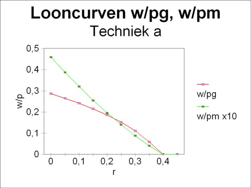
Figure 1: Wage curves for α: w/pg, w/pm
In the two previous columns about the neoricardian theory of Piero Sraffa the equations of the price system and of the material growth have been described. In those columns the production process is given in advance. The present column will explain how the choice of the production technique is brought about. It turns out that the switch to another production process is determined by the shape of the wage curve. The choice for a process is based on the extra-profit, which is predicted by the wage curve of the alternative process. The producer will change his production process, as soon as a more efficient method is found (technological progress), or as soon as the prices of the production factors (labour and capital goods) change.
This paragraph describes once again the price system for a fixed production process. The discussion can be succint, because she has already been presented in the two columns, that have just been mentioned. The determination of the product value is one of the fundamental questions in the history of economics. The classical theory of Ricardo and Marx stranded during the attempt. And later the neoclassical theory of the marginal product experienced difficulties in this respect. The neoclassical thinkers believed that the price system is merely a veil, which covers the real economic phenomena. Then in the last instance each phenomenon in the price system can be simply reduced to the physical effects.
Sraffa shows in his theory, that the price system does create its own effects. There can occur price effects, which can not be explained on the basis of the physical (real) system. Also he reveals the cause of the deviations, namely the distribution of the nett product between the factors labour and capital. Although his theory is fruitful, she is also fairly simple, and in fact little more than conscientious bookkeeping.
In the neoricardian theory of Sraffa the producer j receives for his production a yield according to the formula
(1) pj × Qj = (1 + r) × Σi=1n (pi × qij) + w × lj
The formula 1 does not take into account the time dependency, such as during economic growth. The quantity Qj is the sales of the producer j, qij is the used quantity of product i, and lj is the expended amount of labour. The system contains a total of n products, so that the summation runs from 1 to n. The quantity pi represents the price of the product i, and w is the wage level.
The efficiency r can be interpreted as the rate of profit, that is common in the pervailing social conditions. The interest must be paid from the profit. If it is assumed that the producers do not appropriate the profit, then r equals the rate of interest. Apparently together with the efficiency r there are n+2 unknown variables. The calculation of these variables becomes more transparent, when the quantities are removed from the formula 1. A division of the left- and right-hand side by Qj yields
(2) pj = (1 + r) × Σi=1n (pi × aij) + w × aj
In the formula 2 aij = qij / Qj are the production coefficients, and aj = lj / Qj is the labour coefficient. The n+1 components of the column [aij, aj], which characterize the production process, are called the technical coefficients. The advantage of the presentation in the formula 2 becomes apparent, when the absence of scale effects is posited. When the production on a larger scale does not have (dis-)advantages, then the quantity of the required production factors per unit of product remains equal. Then the technical coefficients are constants, and the formula 2 is a linear equation. Moreover the columns, that have just been mentioned, have shown that the formula 2 does allow to describe certain growth processes.
The producer j can not solve the formula 2 by himself. The prices of his raw materials and equipment are dictated by the market. The solution can only be found at the macro-economic level, where the formula 2 attains the vector form:
(3) p = (1 + r) × p · A + w × a
The matrix A is composed of the production coefficients. Since the set of n equations can not determine n+1 variables, it is common to choose a numéraire. In this column it turns out that the wage level 2 is an appropriate choice, and she transforms the formula 3 into
(4) p / w = (1 + r) × (p / w) · A + a
Now there are n+1 unknown variables, namely pj/w and r. In other words, the pj/w are functions of r. Now the prices are expressed in terms of the wage level.
Considering the eminent importance of the neoricardian theory it is surprising that the supply of accessible text books about the theme is modest. For this column especially the book The production of commodities by J.E. Woods is consulted1. Following Woods an economic system with only two branches is studied, namely the agriculture for the production of corn (in bales) and the industry for the production of metal (in tons of weight). Here the loyal reader recognizes the examples in the previous columns.
The reason for studying the two-dimensional case is that for the more general situation the pertinent effects in the price system can not be visualized in an adequate manner. In such cases is is necessary to analyse the details of the production, partly at the micro-economic level2.
Suppose that each of the two branches can choose between two production methods, namely τ(g1) and τ(g2) in the agriculture, and τ(m1) and τ(m2) in the industry. The table 1 shows the values of the technical coefficients for these four methods. The index j takes on the value g or m, wich refer to respectively the columns for agriculture and industry. Apparently at the macro-economic level four techniques are available, each consisting of a combination of two methods at the branch level. Here the techniques are represented by α = (τ(g1), τ(m1)), β = (τ(g2), τ(m1)), γ = (τ(g2), τ(m1)) and δ = (τ(g2), τ(m2)). In other words, each technique consists of a combination [Aθ, aθ], with θ = α, β, γ or δ.
| agriculture | industry | |||
|---|---|---|---|---|
| τ(g1) | τ(g2) | τ(m1) | τ(m2) | |
| agj | 0.4167 | 0.2727 | 1.290 | 1.60 |
| amj | 0.01667 | 0.09091 | 0.6452 | 0.61 |
| aj | 1.667 | 0.4091 | 3.226 | 6.0 |
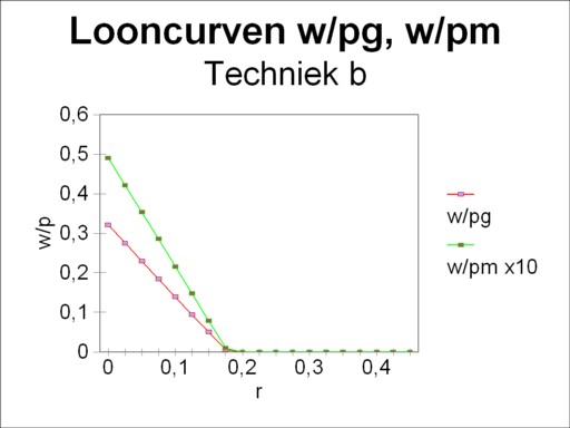
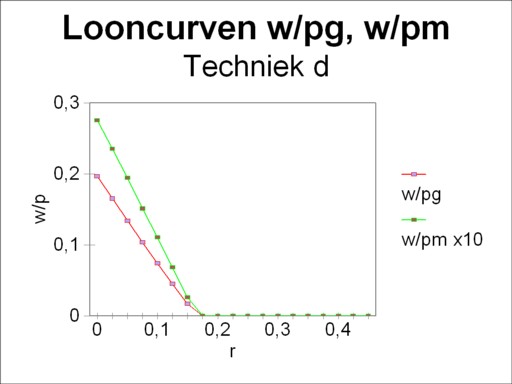
The loyal reader will recognize in the technique α the example from the introductory column about the neoricardian theory of Sraffa. That column shows how the wage curve w/pg(r) can be obtained by means of the matrix calculations. The present column takes an additional step forward. Namely, the choice of the price of corn pg as numéraire is arbitrary. The choice for the price of metal pm is equally justified, which leads to the alternative wage curve w/pm(r). The figures 1, 2, 3 and 4 show these two forms of the wage curve for each of the four techniques α, β, γ and δ. Note that in all figures the wage curve w/pm(r) is scaled up with a factor of 10, for reasons of presentation. In the general case, for each technique there exist as many wage curves as product prices pj.
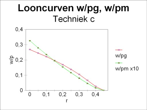
Here it is instructive to compare the four wage curves w/pg. The wage curves w/pg of the technique α and γ have a concave form (the belly points towards the open space). On the other hand the wage curves of the techniques β and δ are convex (the belly points towards the axes). And the wage curves w/pm are convex for the techniques α and γ, whereas they are almost a straight line for the techniques β and δ3.
Each wage curve w/p has the striking property, that she is the reverse of the price p/w, that is to say of the production price, expressed with the wage level as a unit. Apparently the figures 1, 2, 3 and 4 illustrate how the prices vary with the rate of profit r. Thanks to this insight it can now be explained how the producer at the micro-economic level will choose in favour of a certain production process4.
The starting point is that the producer is active for some time, and to be exact in a society that uses the technique α. In other words, the price system consists of [(pg/w)α(r), (pm/w)α(r)]. The index α refers to the fact, that these prices are the result of the corresponding technique. Firstly it will now be argued how the producer will act, when he is a farmer.
The costs of the farmer are
(5) (cg/w)α(r) = (1 + r) × (aggα × (pg/w)α(r) + amgα × (pm/w)α(r)) + agα
The formula 5 is simply the right-hand side of the formula 2, where now all sums are expressed in terms of the wage level w. Here the concept of costs cg is defined in such a manner, that it includes also the profit or the transfer of interest. Then according to the formula 2 the costs equal the selling price (pg/w)α(r).
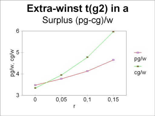
The farmer has the option to change his production process τ(g1) into τ(g2). Incidentally, the figure 2 shows that the method τ(g2) is only viable as long as r is less than 0.178. When r exceeds this value, then the method τ(g2) drops out, and the farmer is inexorably stuck with τ(g1). He wonders what his costs will be for the case of the method τ(g2). He supposes that he will be the only one to switch, which would leave the prices intact. For all of his competitors will determine the market price with their "old" technique τ(g1). With some knowledge about book-keeping he arrives at the conclusiontot
(6) (cg/w)τ(g2)(r) = (1 + r) × (aggτ(g2) × (pg/w)α(r) + amgτ(g2) × (pm/w)α(r)) + agτ(g2)
These costs will almost certainly differ from (cg/w)α. The farmer can obtain a surplus with a size of (sg/w)τ(g2)(r) = (pg/w)α(r) − (cg/w)τ(g2)(r). The farmer can read the numbers (pg/w)α(r) and (pm/w)α(r) simply from the figure 1, and thus he can calculate his surplus. The figure 5 displays the result, by a portrayal of both curves (pg/w)α(r) and (cg/w)τ(g2)(r). Here the surplus is represented by the vertical distance between the curves. Note that in the figure the vertical scale does not start at the origin, in order to accentuate the difference. It is clear that for some values of r the costs are higher than the price of corn. In those circumstances the switch from τ(g1) to τ(g2) would not make sense. But for all profit rates less than 0.024 the switch to τ(g2) yields a surplus above the "normal" profit rate r. In that range of r values the farmer will make the switch.
Now the behaviour of a producer in the industry will be analyzed. In this case the costs are (cm/w)α(r), and they must equal the market price (pm/w)α(r). The producer disposes of the alternative to switch from the production process τ(m1) to τ(m2). Moreover, when r exceeds 0.395, he can no longer produce with τ(m1), and only with τ(mw). See the figures 1 and 3. After the switch the producer has costs with a size of (cm/w)τ(m2)(r). Also this producer can read the numbers from the figure 1, and thus can calculate the range of r values that yield a positive surplus. The switch is worth the effort for values of r above 0.33.
The preliminary conclusion is that the technique α will only be preferred for a rate of profit r between 0.024 and 0.33. Outside this range, either the agriculture or the industry will switch her technique. There does not exist a range where both the agriculture and the industry will switch. The points r=0.024 and r=0.33 are neutral with respect to the profit, when a switch of technique is made. There the producer can employ both alternative methods at the same time. These two points are called the switching points.
The preceding paragraph has explained how the producer will adapt his production method. But this is a solitary action, because it is an individual decision. It seems logical that all producers will imitate his decision, because they also hope to realize the surplus. First consider again the branch of the agriculture5.
Suppose that r is less than 0.024, so that the switch to the production method τ(g2) is profitable. In the situation where all producers have made the switch, they can no longer buy their corn on the market for (pg/w)α(r) nor can they buy metal for (pm/w)α(r). The social production has changed from the technique α to the technique β. The price system which corresponds to the technique β is [(pg/w)β(r), (pm/w)β(r)], and its functional behaviour is illustrated in the figure 2.
In the situation with the technique β the costs for the farmer are
(7) (cg/w)β(r) = (1 + r) × (aggβ × (pg/w)β(r) + amgβ × (pm/w)β(r)) + agβ
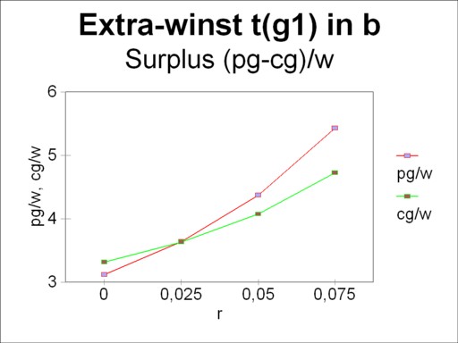
The costs equal the price (pg/w)β(r), so that there is no longer a surplus. Each farmer receives the same common profit. The intriguing question is naturally, whether in the price system of β a single farmer can gain by returning (reswitching) back to the original production method τ(g1). That would initiate a rather unrealistic oscillation.
The figure 6 portrays the curves (pg/w)β(r) and (cg/w)τ(g1)(r), and therefore she is the counterpart of the figure 5. Fortunately now the surplus in the range of r values between 0 and 0.024 is negative. Clearly the option of reswitching does not make sense.
A similar analysis can be made for the situation, where the producers in the branch of industry have adopted the method τ(m2). Then the de facto technique is γ, with her own price system. Also here the reswitching to τ(m1) turns out to be pointless. Lastly it must be noted that the technique δ will never be employed. She is not attractive for anybody.
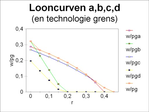
When now the wage curves of the techniques α, β, γ and δ are drawn in the same figure, then the switching points turn out to coincide with the intersections of the curves. This is illustrated in the figure 7, where the vertical axis presents the values of w/pg(r). That is to say, here the numéraire is pg. The envelope of the wage curves is called the technology frontier. Now the precedings arguments have shown, that the producers will always prefer the technique on the technology frontier.
In other words, the minimizing of the costs yields the same results as the maximizing of the wage level (as always expressed in the numéraire). This is a surprising find, which Sraffa discovered thanks to his theory. Thus the technique δ is insignificant, because she never lies on the technology frontier. In the two switching points, namely α-β and α-γ, both price systems yield equal prices6. Therefore it does not matter, which numéraire is selected for the wage curve. It is true that w/pm(r) results in another technology frontier, but the switching points remain equal to those for w/pg(r). The reader may verify this for himself in the figures 1, 2 and 3. This column contains already too many pictures.
The role of the wage curves in the choice of the technology is naturally not really surprising. The largest wage level w/pg for a given r equals the largest nett product for the value of r. And a large nett product offers extra room for profit. Indeed the figure 7 can also be interpreted such, that for a given wage level the technology frontier results in the largest rate of profit r.
The neoricardian price theory of Sraffa leads to several curious effects, which run counter to the common economic intuition. The cause is mainly the habit to identify a rising sum of money with larger physical quantities. In reality a sum of money can also increase due to a raise of the prices. In such cases the common economy states that a price effect occurs, but not a real effect. Obviously sums of money are indispensable, when the value of a collection of goods must be expressed. But one must remain aware, that actually this aggregation of diverse capital goods is an illusion7.
The illusory character of capital aggregation has the consequence, that a redistribution between the incomes from capital and labour will change the production prices in an unpredictable manner. There are no rules of thumb for the development of prices. It is the merit of the neoricardian theory of Sraffa to have shown this effect. But she is not able to identify general price regularities. Those who want to analyze the behaviour of prices, must study the micro-economics of the concerning situation. The present paragraph will attempt to do this8.
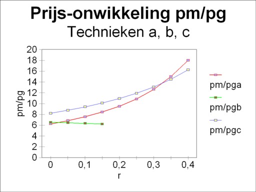
First consider the switch from the technique β to the technique α, for an increasing rate of profit (see the figure 7). The table 1 shows that then the production coefficient agg increases in value, whereas amg decreases in value. That is to say, the producers prefer a method, which per unit of end product uses more corn and less metal. However, when the price development of pg/w and pm/w (or pm/pg, which is more convenient for this case) is studied, then it appears that prior to the switch β→α the metal becomes relatively cheaper. This is shown in a graphic way in the figure 8, in the range r<0.024. On the grounds of this observation it is surprising, that the farmer still prefers a production process with less metal and more corn.
Note that during the subsequent rise of the rate of profit r the producers in the industry make a logical decision. For the switch α→γ implies that agm increases and amm decreases. In other words, henceforth per unit of end product more corn is used and less metal. That choice is reconcilable with the price development of metal, which at that moment rises relative to the corn price. See again the figure 8, but now around r=0.33.
Interesting are also the changes of the labour coefficients ag and am. These represent l/Q, and consequently they are the inverse of the labour productivity9. The switch β→α (r=0.024) is accompanied by a raise of ag, so that henceforth the farm workers will be less productive. That is consistent with the falling wage level. The same can be said about the switch α→γ (r=0.33), where am increases and therefore the workers in the industry become less productive.
This column is concluded with a study of the capital intensities in the agriculture and in the industry10. In general they are defined as
(8) kj = Σi=1n (pi × qij) / lj = Σi=1n (pi × aij) / aj
In other words, the capital intensity represents the sum of production capital per worker. In the present economic example the formula 8 is a system of two equations:
(9a) (kg/w)(r) = (agg × (pg/w)(r) + amg × (pg/w)(r)) / ag
(9b) (km/w)(r) = (agm × (pg/w)(r) + amm × (pg/w)(r)) / am
The capital intensity is a sum of money, and as such it can only display a price effect. Nevertheless it is interesting to see what happens at the switching points. At r=0.024 the switch β→α causes a decrease in kg/w from 7.64 to 1.14. That is convenient for the farmers, in view of the rising rate of profit r. And at r=0.33 the switch α→γ causes a decrease in km/w from 27.2 to 14.4. This will undoubtedly be appreciated by the industry. All in all number of anomalies (unexpected effects) in the present example remain limited.
A fascinating phenomenon, which does not occur in the preceding text, is the so-called reswitching. It concerns a return of the technique, which has already been abandoned at a lower rate of profit (or rate of interest). The reader will understand, that then anomalies are unavoidable. For evidently coefficients aij, which have previously been dismissed, because they were disadvantageous for a rising r, will maintain their disadvantage when they return for an even higher r. Or imagine that a technique with a high labour productivity returns, whereas the wage level keeps falling! The reader may expect a forthcoming column about the reswitching problem.