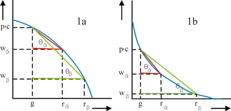
Figure 1: Wage- and consumption curves: 1a concave, 1b convex
In a previous column the neoricardian theory of Piero Sraffa has been explained. An interesting property of this theory is, that she can also model the economic growth. The theory is dynamic. She is directly related to the input-output models of Leontief, and to the matrix formulation of the intertwined balances. It turns out that the growth rate is the dual of the rate of profit.
In this column it is assumed, that the reader already has knowledge about the principles of the neoricardian theory. If desired they can be read over in the previous column, that has just been mentioned. Moreover in the present column the matrix notation is used, so that the detailed description of the system of equations is omitted. The loyal reader of this web portal will probably appreciate that this notation contributes to the transparency of the theory1.
In the column about the intertwined balances the fundamental equation of the neoricardian theory is defined by
(1) ψ(t) = (I − A(t)) · x(t)
The symbol t represents the time variable, and makes the equation dynamic. The formula 1 is a vector equation in n dimensions, where each dimension represents a branch of economic activity. Each branch generates just one product. The quantity in the total product is represented by the vector x(t). The vector ψ(t) is the end product, which is called the nett product by Sraffa.
The difference term I-A shows that the end product is smaller than the total product. Here I represents the unity matrix, and A is the matrix with elements aij = χij / xj. The elements of A are commonly called the production coefficients. The symbol χij indicates the quantity of the product i, which is needed in order to generate a quantity xj of the product j. Apparently in the production coefficients this quantity is reduced to the necessary quantity for a unit of j. Note that the index j refers to both the branch and the product. The formula 1 expresses that a part of the total product is used by the branches themselves.
In the present column the economic growth is introduced in the neoricardian model by taking into account the growth of the population. The growth of the population has the effect, that the professional population l(t) also grows, say with a growth rate g that is constant for all times. Here l is a vector, which describes the distribution of the workers over all branches. It is immediately clear, that the total professional population has a size of L(t) = Σj=1n lj(t) 2. The growth rate indicates that in a time interval Δt the number of workers increases according to
(2) l(t+Δt) = (1 + g) × l(t)
In the present column the formula 2 will be the only source of dynamics. The reader can compare the formula 2 with the model of Solow, and notably the formula 6 there. Now contrary to the model of Solow the technological progress is ignored. There is only one production technique available. In the mathematical formulation this has the pleasant consequence that the production coefficients (and thus also the matrix A) remain constant in time.
The assumption of a single technique implies that per unit of end product j the necessary quantity of labour does not change in time. This quantity of labour is given by the labour coefficients, which are defined by aj = lj(t) / xj(t). Together with the production coefficients they form the technical coefficients. In combination with the formula 2 this means that one has
(3) x(t+Δt) = (1 + g) × x(t)
The formula 3 makes clear that in essence with the passing of time the whole material system scales up according to the growth rate g. Therefore this also holds for the means of production χij(t) and for the end product ψ(t), in all branches. This growth path is called the technically neutral progress.
It is an obvious choice to assume also a constant distribution of income with the passing of time. That is to say, consider the situation where neither the wage level w nor the rate of profit r depends on time. In that case the neoricardian theory describes a form of warranted growth, such as has been defined by the economists Roy Harrod and later Robert Solow3. Then the workers and the capitalists are contented with the status quo. Note that g is also the growth rate of the quantity of "wage goods". This increase will precisely cover the rise of the wage sum, when the wage level is taken constant in time.
In each production cycle (or revolution) the economic system as a whole uses a quantity Σj=1n χij(t) = Σj=1n aij × xj of the product i as a means of production. In matrix notation this is A · x(t). When the cycle lasts for a time period Δt, then in the next cycle the quantity of the means of production must equal A · x(t+Δt) = A · x(t) + g × A · x(t). For the sake of convenience henceforth x(t+Δt) − x(t) will be represented by the symbol Δx(t). Apparently at the start of the new production cycle an extra quantity of the means of production must be available, with a size of A · Δx(t) = g × A · x(t). This quantity must be withdrawn from the end product ψ(t) of the previous cycle.
In the neoricardian theory the additions are called investments
(4) i(t) = A · Δx(t)
It must be admitted that this is somewhat eccentric, because commonly the term investments refers only to equipment. The remainder of the end product is consumed. One has:
(5) C(t) = ψ(t) − i(t)
Apparently the consumption C(t) also grows with the growth rate g. Therefore the ratio cj = Cj(t) / L(t) is a constant quantity. She represents the consumption per capita, and expresses the preferences of the consumers. The reader sees how in this neoricardian model the consumptive needs remain unchanged.
Now the fundamental formula 1 can be rewritten with the help of the other formulas into
(6) C(t) = (I − (1 + g) × A) · x(t)
The formula 6 can be rearranged in such a way, that the solution for the total product is found
(7) x(t) = (I − (1 + g) × A)-1 · C(t)
In the formule 7 the index -1 indicates, that the inverse of the matrix I − (1 + g) × A is meant.
Furthermore note, that by definition the vector of labour coefficients obeys a condition for the mathematical inner product, namely a · x(t) = L(t). Thus the formula 7 can be transformed into a more general form
(8) 1 = a · (I − (1 + g) × A)-1 · c
The interesting aspect of the formula 8 is that all time dependency has been removed. All system variables can be rewritten into unchanged quantities. For this reason the neoricardian model is sometimes called quasi-dynamic. This expression is a bit too condescending.
Incidentally the time dependency can also be removed from the formula 7 without using the inner product. Define the vector η = x(t) / L(t), which represents the total product per capita. The components of the vector η are precisely the inverse of those in a. Since both the total product and the professional population increase with the growth rate g, η will remain unaltered for all times t. Thus the formula 7 reduces to
(9) η = (I − (1 + g) × A)-1 · c
The formulas 8 and 9 show clearly, that the technical equipment imposes boundaries on the options of the consumers. Moreover the options for consumption depend on the economic growth: c = c(g). When the population increases her propagation, and therefore causes a faster economic growth, then she will have to accept a lower level of consumption.
Until now the model only considers the dynamics of the quantities, with the exception of a remark about the distribution of the incomes. The present paragraph discusses the consequences, which result from the value system. For the sake of convenience the formula 6 from the previous column about the neoricardian theory is copied:
(10) p = a · (I − (1 + r) × A)-1 × w
In that column the reader will notice that the set of equations 3a-b is directly normalized by means of the quantities x(t). In this new scale the price system depends only on the unit values, and not on the absolute quantities. In other words, the price system describes merely the exchange proportions, and is independent of the economic growth. This statement is naturally only true, as long as the technical coefficients are indeed independent of the time variable t.
The similarity between the formulas 9 and 10 is striking. In the formula 9 the rate of profit r is replaced by the growth rate g, and the vector a × w is replaced by the vector c, whilst moreover the vector multiplication is introduced on the right-hand side (vertical vector), instead of on the left-hand side (horizontal vector)4. This duality can also be observed in the value expression Y of the end product
(11) Y(t) = p · ψ(t) = p · (I − A(t)) · x(t)
The duality is also found in the formula for the productive capital:
(12) K(t) = p · A · x(t)
On the one hand the formula 12 describes the total sum of profit Π, via Π(t) = r × K(t). On the other hand she describes the value of the investments J, via J(t) = g × K(t). In this way r × K(t) / Y(t) is the constant share of the profit in the end product. And g × K(t) / Y(t) is the constant share of the investments in the end product. In general the profit share and the investment share do not coincide, because the capitalists also consume. They will not accumulate all their profits. Apparently in general the rate of profit r must be larger than the growth rate g. The profit rate r and the growth rate g are equal only in the special case that the accumulation quote equals 1.
In the system of prices the wage curve (r, w) can be calculated simply by using one of the product prices pj as the numéraire for the wage level w. In the previous column about the theory of Sraffa a static system was studied for two dimensions (namely the agriculture and the industry), and the explicit form of w/pg(r) was calculated. There the formula 8 represents a concave curve, which is shown in a graphic manner in the figure 2. It would be interesting to calculate a similar relation for the consumption vector c, which must of course contain g as the argument for the function. However in the system of quantities η the choice for the numéraire is not evident, because the units differ (for instance bales of corn and tons of metal.
The derivation of the consumption curve starts with the assumption, that only one consumption good exists, for instance corn. Suppose that the first branch produces corn, then only the consumption of corn per capita c1 is larger than zero. All other components of the vector equal zero: cj = 0 for j = 2...n. For the sake of convenience define the first unity vector e1 by [1, 0, 0, ... , 0] (a vertical vector), then one has c = c1 × e1.
Thus the formula 8 can be rewritten as
(13) 1 = a · (I − (1 + g) × A)-1 · e1 × c1
The interesting aspect of the formula 13 is, that she is exactly equal to the formula 6 in the previous column about the neoricardian theory, when only the first component of the vector p is considered, and this component is divided by p1 on both sides of the equality. For the result of that operation is
(14) 1 = a · (I − (1 + r) × A)-1 · e1 × w/p1
In the formulas 13 and 14 the duality is perfect. Both formulas describe an identical relation, between on the one hand g and c1, and on the other hand r and w/p1. This means simply, that at least under the assumption of a single consumption good the consumption curve precisely equals the wage curve! This makes the life of an economist a lot easier.
Now an elegant method exists for the analysis of the influence of the rate of profit on the economic system5. This concerns in particular the value of the end product Y(t, r, g) and the value of the productive capital K(t, r, g). The dependency on time disappears when both quantities are divided by L(t). The result is the end product y(r, g) per capita and the productive capital k(r, g) per capita. Other names for these quantities are respectively the labour productivity and the capital intensity.
The end product Y(t) equals r×K(t, r, g) + w×L(t). The division by L(t) gives as a result:
(15) y(r, g) = r × k(r, g) + w(r)
In the same way according to the formula 5 the end product equals g×K(t, r, g) + p1×C1(t, g). Also here the division by L(t) is helpful:
(16) y(r, g) = g × k(r, g) + p1 × c1(g)
The formula 16 shows how the end product per capita depends on the rate of profit r. Since in the right-hand side only k(r, g) depends on r, y(r, g) will behave just like the capital intensity. When k increases, then also y will increase. Obviously this is not surprising. For such a behaviour is typical for production functions Y = F(K, L). In various preceding columns this has already been explained6.
When the right-hand sides of the formulas 15 and 16 are equated, then a formula is found for the capital intensity:
(17) k(r, g) = (p1 × c1(g) − w(r)) / (r − g)
It goes without saying that both the numerator and the denominator on the right-hand side of the equation must be larger than zero. But the formula 17 does not immediately display the variation of k with a changing r. According to the neoclassical theory k must naturally decrease, when r increases. Then the producers prefer the factor labour, which has become relatively cheaper. However, it has already been shown by means of the neoricardian theory, that this neoclassical automatism is an error of thought.
The dependency of the capital intensity on r can best be illustrated in a graphic way. In particular two forms of the wage- and consumption-curve must be considered: the concave shape (see figure 1a) and the convex shape (see figure 1b). It has been stated previously, that the wage- and consumption-curve in the figure 1 must coincide. The horizontal axis represents at the same time r and g, and the vertical axis represents w(r) and p1 × c1(g) 7. It is assumed that the growth rate g remains constant, and then this also holds for the consumption p1 × c1.
But the rate of profit changes from initially rα to a larger value rβ. The consequence is that the wage level falls from wα to wβ. The figure 1 in combination with the formula 17 shows, that the capital intensity must be equal to k(r, g) = tan(θ). To be precise, initially one has kα = k(rα, g) = tan(θα). And after the rise of r she becomes kβ = k(rβ, g) = tan(θβ).
The reader sees how in the figure 1a (the concave case) one has θα < θβ. There due to the increase of the rate of profit r the variable k is raised. This is exactly the behaviour, which is shown in the figure 3 of the previous column about the neoricardian theory. But the figure 1b (the convex case) shows that the reverse happens. Now the increase of the rate of profit diminishes the angle, so that θα > θβ. In other words, k falls. Apparently a priori no statement can be made about the variations of k(r, g) when the rate of profit r changes!
In this final paragraph the dynamic version of the neoricardian theory is compared with the models of the dynamic intertwined balance, which have been discusses previously on this web portal. In the so-called fundamental model the investment formula 4 is replaced by
(18) i(t) = F · ∂x(t)/∂t
In the formula 18 F is a constant matrix. This model has the advantage, that an analytic solution exists.
It is useful to write x(t+Δt) as a Taylor series in Δt, in other words, as x(t) + Δt × ∂x(t)/∂t + (Δt)2/2 × ∂2x(t)/∂t2 + ... The use of this series in combination with the formula 18 yields8:
(19) i(t) = F · Δx(t) / Δt − F · Δt/2 × ∂2x(t)/∂t2 − ...
The formula 19 shows that the neoricardian formula 4 is merely an approximation of the fundamental model. On the other hand, this objection to the neoricardian model is not its refutation: the growth rate is simply g, and that is it. That is to say, the growth is completely exponential (and thus analytic)9. The fundamental model has the additional advantage, that the matrix F is not necessarily equal to A. Therefore the economic system does not need to grow with a general, constant growth rate g. On the other hand, in this fundamental model the price system is naturally absent, and therefore also the economic exchange ratios.
In the so-called model with an investment equation the investment formula 4 is replaced by
(20) i(t) = (A(t) + G(t)) · Δx(t)
So this model does not have an analytic solution. On the other hand, now the matrices of the production coefficients can depend on time, and the depreciation of equipment (that is to say, the use of the fundamental fund) are explicitly and separately registered in the matrix G. Thus in the production process the fixed capital is separated fom the circulating capital.
Moreover the model with investment equation offers the possibility to start the calculations with an arbitrary stock of equipment Γ(0). These aspects make the model factual. But evidently also here the price system is absent, which is so elegantly integrated in the neoricardian growth model. And the solution of this model requires a calculation with steps in time, based on difference equations, which is a cumbersome endeavour.