The falling rate of profit in the labour theory of value

First insertion on Heterodoxe Gazet Sam de Wolff: 15 november 2012

The law of the tendential fall of the rate of profit is an important part of the classical paradigm. Notably Karl H. Marx has made efforts in order to maken this law popular, evidently within the framework of the labour theory of value. In the past decades the law has gained a renewed interest, thanks to the adherents of the temporal single system interpretation (TSSI). Since then Andrew Kliman has published two books about the theory and practice of the TSSI¹. The interpretation has also been discussed on this web portal, in a separate column.

Within the economic science there is some acceptance of the idea, that the rate of profit may fall with the prgression of time. After Marx the English economist J.M. Keynes has studied this phenomenon². The heart of the matter is that the social richness develops in a continuous expansion, and this also holds for the stock of capital goods. Since the growth of the population lags behind, the marginal productivity of capital diminishes. In other words, the investments become less profitable. The availability of capital is more abundant.

The falling rate of profit is called a tendency, because there are countervailing powers, notably the technological progress. Inventions can be a new destination for idle capital, and they can restore its profitability. In the past this has happened during the introduction of the steam engine, the railways, and the motor-car. Nowadays all hope is directed towards the information and communication technology (ICT). See the speculative new economy, and the dot.com bubble in 2001. So although the humans are not powerless, yet the existence of the tendency is credible. For the accumulation of richness is a continuous process, whereas on the other hand the inventions can not be realized on command.

The fall of the rate of profit affects the economic activities. The enterprises can be closed, because the owners are no longer satisfied with their profits. The propensity to invest diminishes, and a stagnation results, or even a crisis and a recession. The result is the stagnation of richness, and therefore a stabilization of the rate of profit. Sometimes the prosperity phase will resume, sometimes not.

Keynes and Marx have different opinions about the possibility to integrate the tendency of the falling rate of profit (marginal productivity of capital) within capitalism. Keynes believes that the state can intervene in order to maintain the investments even in a period of low profits³. On the other hand Marx states that the capitalists will continue their accumulations (investments) at all costs. In each branch only the strongest enterprises will survive the periodic crises. The competition is self-destructive, and finally only the monopolies remain. The state is forced to nationalize them. The present column only discusses the labour theory of value, that is to say, the model of Marx.

The labour theory of value

For the sake of convenience this paragraph gives a succint and schematic summary of the labour theory of value⁴. The labour theory of value has the merit that she contrues a direct relation between the material economy and the price system⁵. Consider an economy with a stock of means of production Pm, a number of workers l, and a total social product Q ⁶. The technical composition T of the capital goods is defined by

(1)     T = Pm / l

T is an indicator of the intensity of the means of production. The technical composition determines the level of the labour productivity ap, which can be written in a mathematical way as ap = f(T). The simplest form of the labour productivity is given by

(2)     ap = Q / l

Subsequently these material quantities must be transformed into labour values. The labour value of the means of production is given by

(3)     c = w_I × Pm

In the formula 3 w_I is the piece value of a unit of means of production. This is the quantity of labour time, which must be expended in order to produce a unit Pm. In a similar way the quantity of necessary labour time v is given by

(4)     v = w_II × w_R × l

In the formula 4 w_II is the piece value of a unit of wage good, and w_R is the number of wage goods, that is given to the worker in exchange for his labour performance. That is to say, w_R is the material wage, and the real wage in the most literal sense.

In the labour theory of value the profit equals the surplus value m. The workers produce an added value N=v+m, which exceeds their wage sum. The producer appropriates the profit. When each worker works for a time τ, then N obtains the value τ×l. Apparently the surplus value is given by

(5)     m = τ × l − v

The rate of surplus value m' can be derived from the quantity m, using the relation m'=m/v. This variable is commonly called the rate of exploitation. The combination of the formulas 3, 4 and 5 allows to calculate the labour value of Q. He is given by

(6)     C' = c + v + m

The formula 6 is valid within an economic system, where the commodities are exchanged in proportions, that match the quantity of labour time, which is expended on each commodity. In the capitalist system the ratios of exchange are modified by the requirement, that the advanced capital must satisfy the general demand for efficiency. Since the advanced sum equals C=c+v (at least within the marxixst model), one has

(7)     r_A = m / C

The quantity r_A is called the general average rate of profit. She is the same for all branches of economic activity. Apparently, in a society with a capital market the formula 6 takes on the form

(8)     Γ' = C × (1 + r_A)

On the macro-economic level (for the system as a whole) C' and Γ' are equal. But at the level of the separate branch i Γ'_i will deviate from C'_i. The labour value is redistributed among the branches.

It is true that the formula 8 modifies the labour value, but still she does not express Q as a monetary sum. This requires knowledge of the so-called monetary expression of labour time ω (abbreviated as MELT). She represents the price of an hour of labour time. Note that the MELT does not coincide with the wage level, because in the labour theory of value the workers do not get paid for their entire working-day. The price sum of Q is equal to p_Q = ω×Γ'. At first sight the introduction of the MELT looks superfluous. However, she does enriche the theory, because she models the influence of money on the system, for instance when the value of money changes. For the sake of convenience the table 1 summarizes the calculation of product prices from the physical quantities.

Economic growth according to Marx

The development of the rate of profit can be understood better, when first the economic growth according to the theory of Marx is explained. This is done in the present paragraph⁷. According to Marx the capitalist system is motivated by the creation of profit, and thus of surplus value. The formula 5 incites the producers to make the variable v as small as possible. The formula 4 shows that the producers can realize their aim by reducing the material wage w_R. However, in the marxist labour theory of value it is assumed that w_R is already pushed down to the minimum level. This idea, which dates from the first half of the nineteenth century, is called the iron wage law. Later it became clear, that in reality w_R has the tendency to rise. Therefore this option is unavailable for the producers.

Nevertheless the formula 4 indicates that v can be reduced, namely by a fall of the piece value w_II of the wage goods. Ignore for a moment the variation across branches, then the piece value in its most general form equals C'/Q. In other words, the piece value can be reduced by increasing the quantity of generated products Q. The formula 2 shows that then for a fixed l of the active (professional) population the labour productivity ap must be enhanced.

It has already been remarked that the labour productivity increases due to mechanization and automation. The technical composition T must grow. The quantity of the means of production Pm must be expanded fast by means of accumulation. That is to say, when the yearly economic rate of growth is g_Q = ΔQ/Q, then the rate of growth g_Pm = ΔPm/Pm must be above average. In a mathematical form the requirement for the two growth rates is: g_Pm > g_Q. Such a development is called a labour saving technical progress. According to the formulas 1 and 2 one has Pm/Q = T/ap. Apparently in this situation the technical composition increases faster than the labour productivity: g_T > g_ap.

When the formulas 1, 3, 4 and 5 are substituted in the formula 7 for r_A, then the following result is found:

(9)     r_A = (τ − w_II × w_R) / (T × w_I + w_II × w_R)

Here the numerator is still the surplus value. Its increase will raise the profit of the producers. However, the formula 9 shows that this attempt will not always be successful. For the behaviour of the denominator is unpredictable. Of course w_I and w_II will fall due to the rising labour productivity, but this development is thwarted by the rapid increase of T.

It is unclear whether the hope of the producers is fulfilled, so that the value of the denominator as a whole will actually fall. It may be just as well, that the rising technical composition will increase the value of the denominator. For it is not easy to maintain a continuous advance of the labour productivity. The rate of profit may fall, much to the dislike of the producers, who accumulate precisely in order to bring about the opposite. Merely accumulating does not score a success. Here is the origin of the law of the tendential fall of the rate of profit in the theory of Marx.

In the past century the law of the tendential fall of the rate of profit has caused a vivid discussion among economists. In an earlier column on this web portal it has already been explained how the whole price transformation of Marx (in the form of the formula 8) has been rejected. The Japanese economist N. Okishio has employed a similar method in order to derive that an increasing labour productivity must by necessity raise the rate of profit r_A. Since then the development of the temporal single system interpretation has turned the tide. The interpretation does not only rehabilitate the price transformation, but she also shows how the rate of profit does fall in a structural way. This phenomenon will be explained in the following paragraphs.

The falling rate of profit in the TSSI: physical growth

The principles of the TSSI have already been described in a previous column. That explanation will not be repeated here. But yet the model will be extended now, because the mentioned column considers only a static economy⁸. The study of dynamics requires that the accumulation process is in fact calculated. For this purpose the paragraph will use an example, which is similar to the one of Andrew Kliman in his book Reclaiming Marx's Capital. Kliman starts with the task of refuting the theorem of Okishio, which states that a rising labour productivity equals a rising rate of profit. This can be done simply by constructing a contradicting case. Incidentally, Kliman states that in such situations the rate of profit will actually always fall⁹.

In order to keep the formalism simple, this paragraph considers an economy with only one branch, and with one product (for instance corn). In this way the complications are avoided, which in a more complete model would emerge due to the intertwined branches. Now the reader also understands why in the introductory paragraph about the labour theory of value the vector notation is renounced. First this paragraph calculates the physical growth. Thus the discussion is confined to the column on the left-hand side of the table 1. In the following paragraph the growth in units of product will be compared with the growth in labour value, by means of the TSSI. See the third and fourth column in the table 1.

Suppose that the labour productivity ap rises with a constant growth rate g_ap = Δap(t)/ap(t-Δt). Here t represents the time variable, and Δt is the time interval that changes ap. The number of workers l and their real wage w_R are kept constant in time. For the sake of convenience it is assumed that all physical surplus value M(t, Δt) is used for accumulation. Here the time interval Δt indicates the duration of the production process, which creates the surplus value. The reader must not confuse M(t, Δt) and the surplus value m in labour values! The profit is added as a whole to the stock of capital goods, or in other words, the accumulation quote equals 1. Thus one has the formula

(10)     ΔPm(t+Δt) = M(t, Δt)

In the formula 10 ΔPm(t+Δt) is defined as Pm(t+Δt) − Pm(t). That is to say, the increase ΔPm takes place at the end of the time interval Δt.

Since there is only one product, the physical means of production and the physical wage sum can be simply added. So this extremely simple economic system can be calculated in terms of the physical quantities. The result is

(11)     Q(t+Δt) = Pm(t) + w_R × l + M(t, Δt) =
             Pm(t+Δt) + w_R × l

In the second step the fomula 10 is inserted. According to the formula 11 the total social product is expended on the advance of capital for the next production cycle (revolution period). She shows directly how Q changes with time

(12)     ΔQ(t+Δt) = ΔPm(t+Δt)

Figure 1: Physical development

Moreover the formula 2 implies that the growth rate of Q satisfies ΔQ/Q = g_ap. The combination of this expression with the formula 12 yields

(13)     ΔPm(t+Δt) / Pm(t) = g_ap × Q(t) / Pm(t)

The formula 13 shows that the rate of growth g_Pm of Pm is larger than the one of Q. Apparently the exclusive accumulation in the stock of the means of production causes a labour-saving growth. Incidentally during the continuing accumulation the fraction Q(t) / Pm(t) will approach 1. So the asymptote is g_Pm = g_ap.

Finally for this simple economic system it is possible to find the physical rate of profit. She is defined by r_M(t, Δt) = M(t, Δt) / (Pm(t) + w_R × l). Substitution of the formulas 10, 11 and 12 yields

(14)     r_M(t, Δt) = ΔQ(t+Δt) / Q(t)

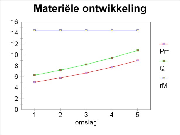
The formula 14 shows immediately how r_M behaves. For the right-hand member is equal to g_ap, and this is by assumption a constant. The conclusion must be that in the given conditions r_M(t, Δt) is a constant as a function of time¹⁰. The figure 1 is an example, which illustrates the development, and she is calculated with the parameter values at the end of this column.

The falling rate of profit in the TSSI: value growth

To begin with it may be useful to point out that in the preceding paragraph the time period Δt of the production process plays a vital role. This is the hallmark of the TSSI. In other so-called simultaneous calculation methods it is assumed that the production process is completed almost instantaneously. In such methods the time between two production cycles (revolutions) is essential. On the other hand, in the TSSI the time between two cycles is not important. It is assumed that the producer will invest his yield immediately in order to start the next cycle (revolution). The assumption of the TSSI seems credible.

The assumption of an economy with only one product and one branch eliminates the problem of the value modification at the level of the branches. There is no redistribution of value between branches. In this case the value modification is simply a change of formulas. The formula 6 can be transformed into the formula 8. The columns 2 and 3 of the table 1 coincide.

The MELT ω is taken to be constant, and put equal to 1, because she is irrelevant for the present arguments. Then the modified labour values are equal to the money prices. The columns 3 and 4 in the table 1 coincide. The computation of the labour values has already been described in the formulas 3 up to and including 8. In a one product economy there is naturally only one piece value w(t). Besides, now the formulas must take into account the time dependency. For instance the formula 6 in full is

(15)     C'(t+Δt) = c(t) + v(t) + m(t, Δt)

Figure 2: Value development

Now the crucial question is how the rate of profit r_A in units of labour value behaves. For the present application it is common to use the formula 7. More information can be derived by an alternative formulation, namely¹¹

(16)     r_A(t, Δt) = r_M(t, Δt) × (1 + g_w(t+Δt) × (1 + 1 / g_ap))

The advantage of this alternative formula is that the relation with the physical rate of profit r_M becomes visible. Moreover she contains the growth rate g_w(t+Δt) = (w(t+Δt) − w(t)) / w(t), which expresses the effect of the rising labour productivity. This growth rate is negative, because w(t) decreases with time. Thus it can immediately be concluded, that r_A is smaller than r_M. Apparently the TSSI leads to a different result than the method of Okishio, which predicts equal rates of profit in both cases.

For cases where t is sufficiently large, the formula 16 can be simplified. For this purpose it is convenient to simplify the expression somewhat¹²:

(17)     r_A(t, Δt) / r_M(t, Δt) = (m(t, Δt) / C'(t)) / g_ap

The formula 5 shows that the surplus value can never exceed N=τ×l. Due to the accumulation C'(t) can be raised to an arbitrary level, and finally it will significantly exceed N. Apparently the formula 17 predicts a continuous fall of the ratio r_A(t, Δt) / r_M(t, Δt) with the progression of time. It is regrettable that Kliman does not elaborate on this point in his book Reclaiming Marx's Capital. Nor does your columnist find any texts on the world wide web, that shed light on this matter. There remains yet work to be done with regard to the TSSI.

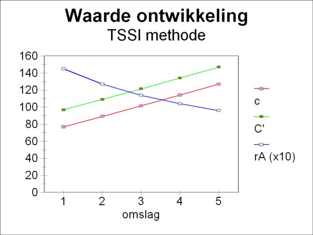
Nonetheless, all examples, that your columnist has seen, show a falling rate of profit in labour values. The figure 2 illustrates this phenomenon, and is calculated with the parameter values at the end of this column.

An example with the TSSI

Columns on this web portal have the habit to end with an illustrative example, and this column follows suit. The table 2 contains the values of all the quantities, that are needed for the calculation. They can be made lively by assuming that the numbers portray for instance bales of corn. At the start of the first revolution (t=1) 5 bales of corn are available for sowing. The farm workers are paid with an aggregate wage sum of 0.5 bales of corn. Apparently a total of 5.5 bales of corn is available as an advance. This quantity could originate from a previous revolution with a yield of 5.5 bales of corn. The growth rate of the labour productivity predicts that at the end of the first revolution (for instance at the yearly harvest) a yield of 6.3 bales of corn will be available. Apparently the physical surplus value M is 0.8 bales of corn.

The further development of the system can be calculated with the formulas 2 and 10. The table 3 shows the development of the most important physical quantities. The figure 1 shows the results in a graphic manner.

Subsequently the development of the labour values is studied. The formula 16 shows a typical property of the TSSI, namely that the calculation can only be done when the piece value w(1) at the start of the first revolution is known. The recursive character requires an initial condition. This value must be chosen, for instance w=15.4 labour years for each bale of corn. However, the value can also be made credible by means of a historic argument. Suppose for instance, that in previous times the labour productivity has always been constant. In other words, in the past the economic system reproduced itself. Each year 5.5 bales of corn were advanced, and 6.3 bales of corn were produced. The nett product was 1.3 bales of corn in each year. According to the formula 5 the labour value of this nett product equals N=τ×l. Suppose that τ has the value of 1 (working-year). Then the piece value of a bale of corn is w = N/(Q-Pm) = 20/1.3 = 15.4.

Now suppose that at the end of the first revolution the producers change the system into capitalism with accumulation and growth (extended reproduction), in the way that has been described in the previous two paragraphs. The accumulation quote equals 1, etcetera. The labour productivity rises, and the piece value falls. At the end of each revolution the piece value is

(18)     w(t+Δt) = C'(t+Δt) / Q(t+Δt)

So the w in the formula 18 is the piece value directly at the end of each revolution, at the moment when the total product is sold. Since the producers use their yield immediately in order to advance the capital for the next revolution, this w is also the piece value at the start of that revolution.

The labour values of the various quantities can be calculated from the table 3 for the revolutions 2 up to and including 5, by using the initial condition w(2) and the formula 18. Here the rate of profit r_A is calculated simply as m/C. Thus the development in labour values (and in money, due to ω=1) is found, and the result is shown in the table 4. The figure 2 shows the results in a graphic manner. Note that for reasons of presentation the rate of profit in the figure is scaled up by a factor of 10. The table 4 shows how the rate of shrinkage g_w becomes more negative with the progression of time. According to the formula 16 this influences the time behaviour of r_A. The rate of profit in labour values falls, just as is predicted by the marxist law.

1. The theory of the TSSI is explained in Reclaiming Marx's Capital (2007, Lexington Books). The application of the theory in the American economy is described in The failure of capitalist production (2012, Pluto Press). Both books are fairly accessible for those interested, with an average education. (back)
2. An excellent comparison of these two thinkers can be found in Marx and Keynes (1980, Merlin Press) by Paul Mattick. The following arguments are mainly copied from this book. See p.15 and further, and also p.109 and further. Mattick was active as a political economist. (back)
3. Mattick writes on p.112: Keynes was convinced that "a somewhat comprehensive socialization of investments will prove the only means of securing an approximation of full employment", but "this need not exclude all manners of compromise and of devices by which public authority will co-operate with private initiative". Only experience would show, he thought, "how far the common will, embodied in the state, ought to be directed in increasing and supplementing the inducement to invest; and how far it is safe to stimulate the average propensity to consume". (back)
4. For a more precise exposition, see the column about the transformation problem. (back)
5. The arguments that now follow are taken from the book Die Marxsche Konjunkturtheorie (2009, PapyRossa Verlag GmbH) by Alfred Müller. This book is highly recommendable for economists with an interest in the marxist paradigm. It employs the peculiar approach to analyze mainly the changes of quantities, instead of their absolute values. The arguments can also be found in the reader Voortgang der economische wetenschap (2011, Uitgeverij E. de Bibelude) by E.A. Bakkum. (back)
6. This notation serves only to sketch the scheme. In fact Pm is evidently a vector of all the available means of production, and Q is a vector of all the generated end products. (back)
7. Also this paragraph is inspired by the explanation in Die Marxsche Konjunkturtheorie. (back)
8. Nevertheless an example in the pertinent column has shown that in this situation the general average rate of profit is not necessarily constant. For the price transformation implies a continuous value modification, in the manner that is shown in the table 1. Thus in the example the rate of profit approached the value zero. This is an intriguing aspect of the TSSI, which can not be excluded in advance. There are valid arguments for the assumption, that this effect will be weakened in reality. For instance the analytic concept of the general average rate of profit is just an abstraction. For it is common that the rate of profit varies, depending on the particular branch. (back)
9. The example of Kliman can be found on p.127 and further in Reclaiming Marx's Capital. The statement that in fact the rate of profit is always falling, is repeated again on p.206. Unfortunately Kliman does not provide a formal proof. Evidently a single example can not replace that proof. Your columnist will address this matter presently. (back)
10. The example of Kliman on p.121 of Reclaiming Marx's Capital has a rising physical rate of profit r_M. Even then the TSSI method yields a falling rate of profit r_A in labour values. The example in paragraph 8.9.3 of Vooruitgang der economische wetenschap also has a rising r_M. The increase is caused by the assumption of a constant w_R + M/l instead of a constant growth rate ap=Q/l. In other words, in those examples the constant labour productivity pertains to the nett product, that is to say, on the newly created physical matter. This is the definition of labour productivity, which is common in empirical studies. The reason for the use of the alternative definition is, that it is more difficult to determine the seize Q of the total product instead of the seize of the newly created product. For the present application this is irrelevant. For here the aim is to illustrate, that the rate of profit r_A falls, even when the rate of profit r_M does not. (back)
11. The formula 16 is derived as follows: r_A(t, Δt) / r_M(t, Δt) = m(t, Δt) / C(t) × (Pm(t) + w_R×l) / M(t, Δt) = m(t, Δt) / (M(t, Δt) × w(t)) = (C'(t+Δt) − C(t)) / (ΔPm(t+Δt) × w(t)) = (Q(t+Δt) × w(t+Δt) − Q(t) × w(t)) / (ΔPm(t+Δt) × w(t)). Substitute Q(t) = Q(t+Δt) − ΔQ(t+Δt) en ΔQ(t+Δt) = ΔP(t+Δt), then the result is r_A(t, Δt) / r_M(t, Δt) = 1 + Q(t+Δt) × Δw(t+Δt) / (ΔQ(t+Δt) × w(t)) = 1 + g_w(t+Δt) × Q(t+Δt) / ΔQ(t+Δt) = 1 + g_w(t+Δt) × (1 + 1 / g_ap). Thus the derivation is completed. (back)
12. The formule 17 is derived as follows: r_A(t, Δt) / r_M(t, Δt) = m(t, Δt) / (M(t, Δt) × w(t)) = m(t, Δt) / (ΔPm(t+Δt) × w(t)) = m(t, Δt) / (ΔQ(t+Δt) × w(t)) = m(t, Δt) / (g_ap × Q(t) × w(t)) = (m(t, Δt) / C'(t)) / g_ap. Thus the derivation is completed. (back)