Figure 1: Production set
-- with profit maximization
Many columns on this webportal discuss the input-output model of Leontief. The characteristics of the Leontief model are the constant returns to scale, labour as a separate production factor, and the absence of coupled production. In fact it is a linear model and thus a special case of the economic theory of capitalist production. In the general theory also non-linear production processes can be described. Then it is convenient to formulate the theory in terms of algebraic sets. The present column aims to integrate the algebraic set in the common Leontief model. The text is based mainly on the book Micro-economic theory van A. Mas-Colell, M.D. Whinston en J.R. Green1.
The open Leontief model consists of a set of vector equations
(1a) y = (I − A) · x
(1b) L = a · x
In the set 1a-b x is the vector of product quantities. When the system contains n different products, then x has n components. The vector y represents the size of the nett- or end-product. The scalar L is the quantity of labour time, which has been expended during the production.
The matrix A consists of constant elements aij. They express the quantities of the products i (with i=1, ..., n), which are needed for the generation of a unit of product j. These numbers are called the production coefficients. The components aj of the vector a express the amount of labour time, which is expended for the production of a unit of product j. They are called the labour coefficients. The elements of A and a together are called the technical coefficients. The symbol I represents the unity matrix. The reader can find a more detailed explanation in a previous column.
The set 1a-b can be written in the form
(2a) yi = Σj=1n (δij − aij) × xj
(2b) -L = Σj=1n -aj × xj
In the formula 2a-b Σ is the mathematical symbol for summation, in this case with j=1, ... , n. The symbol δij is the Kronecker delta. This set is suited for an explanation of the algebraic concept of sets in the production theory.
First define the so-called elementary activity j, which belongs to the product j. She is represented by a vector α(j) in the n+1 dimensional space. Its components are
(3a) αi(j) = δij − aij voor i= 1, ... , n
(3b) αn+1(j) = -aj
In fact α(j) is simply the j-th column of the matrix I − A, extended by the component aj in the lowest row.
Next define an arbitrary production activity. She is represented by a vector η in the n+1 dimensional space. Its components are ηi = yi for i= 1, ... , n, and ηn+1 = -L. In other words, η is the vector of the nett product, extended by the amount of expended labour in the lowest row. Since labour is consumed, this last component is negative. Together with the sets 2a-b and 3a-b the definition leads to
(4) η = Σj=1n xj × α(j)
It is immediately clear from the set 3a-b, that each elementary activity contains a number of negative components. The economic meaning of this phenomenon is, that production factors enter the production process and are consumed. Therefore also the production vector η can have negative components. It is obvious, that in an economically meaningful vector of production at least one component must be larger than zero. For only then the process yields an output. In case that all components are zero, the production is inactive. She is shut down.
Nevertheless a completely negative vector in possible, in principle. For the sake of convenience the elementary activities are complemented with the so-called disposal activities d(j). These vectors have the value -1 as j-th component, and zero for the other components. That is to say, d(j) = -e(j), where e(j) is the unity vector for the j-axis. A branch j can only generate its product, as long as sufficient production factors are available from the other branches. Production vectors η, which can not be realized by the existing technique, are not part of the set Π. But an excess of production factors can be disposed of by means of the disposal activities.
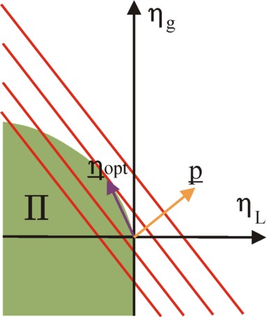
Perhaps the reader will wonder whether this theory of algebraic sets serves a useful purpose. The advantage is that within this theoretical frame the optimal production vectors can be found. As an illustration the figure 1 shows a set Π for the production of corn. She corresponds to the green area. The corn is both seeds for sowing (a production factor) and end product. A nett product ηg is generated. Besides corn the production process requires only the input of a quantity ηL of labour time. In other words, the production vector is two-dimensional, with components η = [ηL, ηg].
The production method in the agriculture puts boundaries on the harvest, because she corresponds to a certain labour productivity ap. It is obvious that a maximal output of corn is preferred, for a given amount of labour time. Therefore the production vectors on the upper boundary of the set Π are called optimal or efficient2. However, also all vectors below this boundary, in the green area, are possible and are part of Π. Note that the area with positive values of ηL is excluded from Π. It has already been remarked, that ηL must be negative. This is always the case. For the factor labour itself can not be produced (at least in this model). Therefore labour time is called a primary factor3.
The production vector is well suited for the calculation of the profit φ of the producer. Namely, let pj be the market price of the product j. Then the whole price system can be represented by the vector p with components pj (j=1, ... , n) 4. And the profit is given simply by the inner product
(5) φ(p) = p · η
In the formula 5 use is made of the fact, that the production factors in η are presented as negative numbers. Note, that the profit depends on the price system. As an illustration in the figure 1 several iso-profit curves are drawn. These are lines, which connect the production vectors with a single and constant profit φ. The angle between the price vector and these lines is rectangular5.
For a given price system p the problem of profit maximization is given by
(6a) maximize p · η
(6b) under the condition η ε Π
In the formula 6b ε represents the "is an element of" sign. The figure 1 shows immediately, that the vector, which maximizes the profit, is given by the isoprofit line, which is just the tangent of the upper boundary of the set Π. The point of contact is the optimum6.
The advantage of the theory of production sets is that she also holds for production methods, which are not linear. Whereas the Leontief model is merely applicable to the case of constant returns to scale, the theory in the present paragraph is also applicable for positive or negative returns to scale. In other words, the theory can be applied in a broader manner than merely in situations with production vectors that obey the formula 4. The technical coefficients do not have to be constants. At the same time the importance of this advantage must not be exaggerated. For instance the positive scale effects suggest, that the profit can be increased at will be a continuous expansion of the production. But this does not allow for an optimization, which is the aim of the economic theory.
In addition to the mentioned advantage the theory of the production set allows to include coupled production. The production vector of a single branch can contain two or more positive components. And it is convenient, that separate production vectors can be simply added (aggregated). When the production vector of the society as a whole is considered, so at the macro-economic level, then η can not contain any negative components (with the exception of labour time). For in this situation a negative component implies, that the society has a shortage of the pertinent production factor. That deficit must be covered by stocks, and that is not a durable solution.
As an illustration of the preceding two paragraphs the familiar example of an economy with two branches (n=2) is again analysed, namely the agriculture (branch 1) and the industry (branch 2). In the agriculture 20 workers (20 units of labour time, lg = 20) generate 12 bales of corn (xg = 12) during a production period. In the industry 10 workers (10 units of labour time, lm = 10) generate 3.1 tons of metal (xm = 3.1) during the same production period. The nett or end product is y = [3, 0.9].
The production technique is determined by the technical coefficients. The values of those coefficients aij and aj are presented in the columns τ(g1) and τ(m1) of table 1. Moreover the table contains an alternative production method for the agriculture, which is presented in the column τ(g2). Now the set 3a-b can be used in order to transform each of these three methods into an elementary activity.
| agriculture | industry | ||
|---|---|---|---|
| τ(g1) | τ(g2) | τ(m1) | |
| corn | agg=0.4167 | agg=0.2727 | agm=1.290 |
| metal | amg=0.01667 | amg=0.09091 | amm=0.6452 |
| workers | ag=1.667 | ag=0.4091 | am=3.226 |
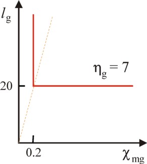
The elementary activity of τ(g1) is the vector [0.5833, -0.01667, -1.667]. Now the formula 4 can be used for the calculation of the production vector, which generates for instance a gross (total) product of 12 bales of corn. In other words, it is possible to calculate the vector, which corresponds to a level of 12 bales of corn. The result is the production activity [7, -0.2, -20]. So 7 bales of corn are produced7, and this process consumes χmg = 0.2 tons of metal and lg = 20 units of labour time.
It may seem that in the plane (χmg, lg) the isoquant of these 7 bales of corn consists of a single point [0.2, 20]. However, contrary to the Leontief model the production set allows for production plans, which are not efficient (see for instance the figure 1). The same 7 bales of corn can be produced with larger quantities of the production factors factoren χmg and lg. For the producer can employ disposal activities, which allow to remove the excess of production factors. Therefore the isoquant for 7 bales of corn has the shape of the figure 2.
A special property of the isoquant in the figure 2 is, that the substitution of production factors is impossible. This is the hallmark of a production method with constant technical coefficients. Consequently the producer can not adapt his production process in a flexible manner to possible price changes of the production factors. Moreover a possible expansion of the production must follow the path of the dotted line, because the process scales in a linear manner8.
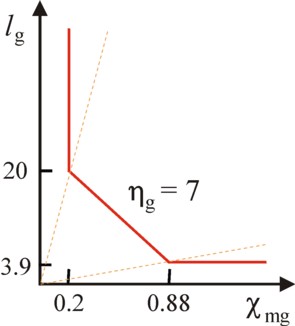
A more interesting case occurs when two elementary activities generate the same product. For instance, suppose that the agriculture can also apply the method τ(g2), with production vector [0.7273, -0.09091, -0.4091]. Also this method can generate a nett product of 7 bales of corn, albeit with a level of activity equal to 9.625 bales of corn. The necessary quantities of production factors are χmg = 0.8750 tons of metal and lg = 3.937 units of labour time.
The figure 3 shows the isoquant for 7 bales of corn after the inclusion of the elementary activity τ(g2). This activity obviously adds the point [0.8740, 3.937] to the isoquant. But because of the formula 4 also all production vectors on the line piece between the two points [0.2, 20] and [0.8740, 3.937] are possible. The situations on this line piece do allow for the substitution of the production factors!
Unfortunately the substitution is useless. Namely, a so-called non-substitution theorem can be proven, which limits the number of efficient production vectors9. According to the theorem, all efficient production vectors in the presented example with two products (bales of corn and tons of metal) can be generated with exactly two elementary activities. There is no need for a third elementary activity, such as in the table 1.
The loyal reader of the Gazette will not really be surprised by the non-substitution theorem. For in a previous column about the neoricardian production theory is has already been explained, that for each wage level pL only one technique has a maximal efficiency. The column, just mentioned, shows for the present example, that the method τ(g2) is more efficient for pL/pg > 0.277, whereas conversely the method τ(g1) is more efficient for pL/pg < 0.277. Merely in the point pL/pg = 0.277 each linear combination of both production methods can be chosen, without negative consequences for the efficiency. Apparently the line piece of the isoquant corresponds with the price vector, which belongs to the switching point of the two techniques.
This paragraph is an elaboration of the properties of the input-output tables. For the sake of completeness it helps to remind the reader, that the former planned economies in Eastern Europe preferred to use the expression intertwined balances. The formula 4 shows that the elementary activities α(j) form a set of basis vectors, as it were, which can be combined to express all kinds of production plans η. However, when efficient production vectors must be expressed in terms of the α(j), then those particular elementary activities must be selected, which for the given price system p indeed maximize the profit. When an α(j) generates a loss, then she is not eligible.
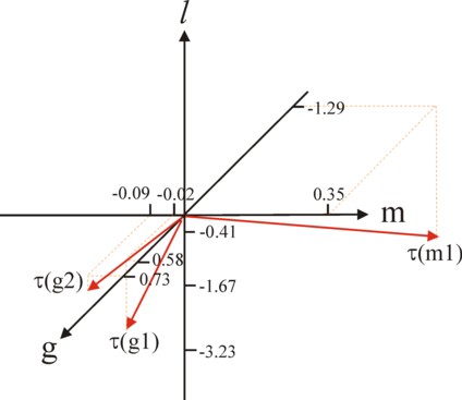
The role of the elementary activities can be illustrated by means of the example, which has been introduced in the preceding paragraph. There three elementary activities are described, namely α(g1) = [0.5833, -0.01667, -1.667], α(g2) = [0.7273, -0.09091, -0.4091], and α(m1) = [-1.29, 0.3548, -3.226]. These are vectors in the three-dimensional space. Although it is a difficult endeavour, your columnist has tried to draw them in the figure 4.
In the figure the three-dimensional crossing of axes is represented by the black lines. The arrows mark the positive part. The quantities of corn and metal are displayed in the horizontal planes. The labour time l is measured on the vertical scale, where naturally only the negative part of the axis has a real meaning. The red vectors correspond to the elementary activities. Dotted lines are used in an attempt to express the spatial perspective of the arrows within the crossings. All three vectors poins downwards. Furthermore, the agricultural activities point in the left-forward direction, whereas the industrial activities point in the right-backward direction.
In the preceding paragraph it has been explained, that for the wage level pL/pg > 0.277 the efficient production vectors lie in the plane, which is spanned by the vectors α(g2) and α(m1). However, when the wage level is pL/pg < 0.277, then the efficient production vectors lie within the plane of the vectors α(g1) en α(m1). The reader may remember, that the levels xj of the activities can not be negative. Therefore the possible production vectors η are completely "wedged in" by the two spanning elementary activities.
Finally, it is worth mentioning, that the concept of the elementary activities has a practical meaning. The Russian Leninist economist V.V. Kossov points out in his book Verflechtungs-bilanzierung, that the design of the input-output tables always requires some aggregation of the various branches10. The aggregation prevents the bulging of the tables or matrices, which would impede the performance of calculations. Besides a detailed data collection is often impossible, simply because the empirical data are unavailable.
Next a choice must be made for the branches, which are preferably aggregated in the process of simplification. The aggregation is only meaningful, if the concerned branches have much in common. Apparently a criterion is required for the classification of the branches according to their technical properties. Kossov proposes to aggregate branches, which use approximately the same production factors, in approximately equal proportions. Moreover the end products of the aggregated branches must bear some resemblance. In other words, those elementary activities must preferably be aggregated, which have their vectors pointing in approximately the same direction.
The approach of aggregation, mentioned just now, can be illustrated by means of the example. Two vectors point in approximately the same direction, when their angle θ is small. And θ can be found simply by calculating the inner product of the two vectors11. Thus it is computed that the angle θ between α(g1) and α(g2) is 41.6°, between α(g1) and α(m1) it is 41.5°, and between α(g2) and α(m1) it is 83.2°. Apparently the aggregation of the two productions of corn almost matches the aggregation of τ(g1) in the agriculture and the industry.
This conclusion may surprise, certainly when the figure 4 is considered. The two agricultural activities seem to almost coincide, but the point of view is somewhat misleading. Moreover the scales of the axes are not equidistant. The scales on the axis of corn and especially the scale for the axis of metal are stretched. However, a closer examination reveals that α(g2) has a rather low intensity of labour. Reversely, both the industry and α(g1) in the agriculture are rather labour-intensive. That could indeed be an argument in favour of the aggregation of two seemingly different branches. After such a choice for the closest branches, the practical aggregation is naturally done with the help of the formula 4.