Dynamics in macro-economic production functions
First insertion on Heterodox Gazette Sam de Wolff: 31 march 2014
E.A. Bakkum is a blogger for the Sociaal Consultatiekantoor. He loves to reflect on the labour movement.
Until now this webportal has somwhat neglected the neoclassical production theory. The present column makes up for this omission by describing the micro-economic theory of production functions. Essential concepts such as the complementarity and the substitution of production factors are explained. The isoquant is introduced, as well as the occurrence of various types of scaling effects. The problems of macro-economic production functions, such as in the model of Solow, are addressed. Although the theory in this column remains at the introductory level, she is useful and even indispensable for future columns about the technical development in the production1.
The micro-economic production function
When in an enterprise a quantity Q of some good or service is produced (output), then production factors are required (input). The production factors are quite diverse, and vary from labour, raw materials, expedients and semi-manufactured articles to the machinery and the buildings. Suppose that N of such factors exist, with their corresponding quantities given by the set (q1, q2, ... , qN). Together the quantities form an n-dimensional vector q. Now the production function is defined as the function Q = f(q), which describes the relation between the inputs and outputs2.
The production function is a typical find of the neoclassical paradigm, which tries to describe the economy at the micro level of the enterprises and the households. The function is an abstract representation of a certain production process or enterprise. That is to say, she symbolizes a certain production technique. The variables refer to the material situation, and ignore the monetary value of the production factors and of the products. The choice for a production function is made by the entrepreneur himself. In the current theory the organizational, managerial and administrative regulations are not explicitely mentioned in the formulation of the production function3. She does admit, that the environment of the entrepreneur affects Q. Since the approach is neutral with respect to the system, Leninist economists do not make ideological objections against the use of production functions.
It is commonly assumed, that f(q) describes a technically efficient production. The quantities qi (with n=1, ..., N) are completely employed. For although in f(q) the value is absent, the neoclassical paradigm does require that the costs are minimized. Moreover, since she expects that the products are sold at their heighest prices, she defines the problem of the entrepreneur as4
(1) maximize for the q-space f(q) × p − Σn-1N qn × pn
In the formula 1, p is the product price, and pn is the factor price of the input n. It is obvious that the production is merey viable, as long as the difference between the benefits and the costs is positive. In the situation with pure competition the entrepreneur can not influence the prices, so that he becomes a price taker, who adjusts the quantities. The choice for a certain volume Q of production is dictated by the behaviour of f(q). For the sake of convenience the economists like to use in their models the so-called homogeneous production functions of degree γ, that satisfy the relation
(2) λγ × Q = λγ × f(q) = f(λ × q)
In the formula 2, λ is a real number, which allows to scale the production volume in upward or downward direction. This is called the level variation. Insertion of the formula 2 in the formula 1 gives5
(3) maximize for the q-space q1 × { q1γ-1 × f(q / q1) − (q / q1) · (p / p) }
In the formula 3 the last term represents the mathematical inner product of the vectors q/q1 and p/p. The formula 3 is written in such a manner, that q1 is a scaling factor, whereas the ratio qn/q1 represents the technique.
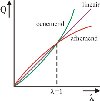
Figure 1: various scaling effects
The formula 3 does not imply, that q1 must be maximized. That depends on the value of the term Ψ(q1, q/q1) = q1γ-1 × f(q / q1) − (q / q1) · (p / p). A special case occurs for γ=1, because then Ψ depends only on the technique, but not on q1. Note that in this situation one will have Ψ=0 6. The case γ=1 has apparently the hallmark, that the maximization does not depend on the scale of the production process ( constant returns to scale). This type of production functions with γ=1 is called linear-homogeneous.
On the other hand there are positive scaling effects (increasing returns to scale), when one has γ>1 (more-than-linear). For, then a given technique q/q1 has a positive Ψ for an increasing q1, due to the rising term q1γ-1 × f(q / q1). Such a situation furthers the formation of monopolies, so that the perfect competition will be undermined. The case γ<1 (less-than-linear) has negative scaling effects. The formula 3 shows that in this case an increasing scale of production will finally lead to a negative Ψ and thus to losses for the enterprise. Here the entrepreneur must try to find the optimal volume of production Q = Qopt. The figure 1 displays in a graphical manner the behaviour of the production volume as a function of the scaling factor λ, for the three regimes of γ.
The basic model of the neoclassical paradigm assumes a perfect competition, and therefore chooses a linear-homogeneous f(q). Unfortunately, this is not very realistic. Besides, the figure 1 already suggests, that none of the homogeneous production functions is universally applicable (not even with γ<1 or γ>1). In general, the reality is a mix of those cases. Notably for a small volume of production an increased scale is beneficial due to the falling costs per unit of product, because some production factors are not divisible. Consider especially the "fixed" costs, such as the administration, which is necessary even for Q=0. On the other hand, the services often exhibit a neutral scaling. The fixed costs are small.
Reversely, a very large scale can lead to a rigid and expanding bureaucracy, which stifles the efficiency. Incidentally, the neoclassical paradigm can not explain this latter phenomenon. In its perspective the conflicts of interest within the organization are ignored. There are no conflicts of target. Furthermore, due to exhaustion all kinds of mining and reclamation on a large scale will often suffer from decreasing surpluses. Anyway, this shows that in the true production function the scaling effects can change, depending on the volume of production. In reality an increased scale will sometimes even be accompanied by the selection of a completely different production function.
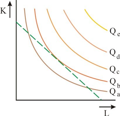
Figure 2: Isoquants with budget line
When the behaviour of the production functions is studied, the isoquants are a useful aid. They are defined by the equation Q0 = f(q), where Q0 represents a constant value. A fascinating question is whether the function allows to produce Q0 with various vectors q, for instance with q1 and q2. When this is impossible, then the proportions qn/qm are apparently fixed in advance. Production factors with this behaviour are called complementary. The factor intensities qn/qm are fixed, and thus also the production coefficients qn/Q0. The isoquant is simply a point in the q space. These are called limitational production functions or Leontief production functions7.
The neoclassical paradigm is not interested in complementary production functions. For, it describes the behaviour of the entrepreneurs by means of the formula 3. The entrepreneur searches for the production functions with the lowest prices pn. In the neoclassical perspective he is always sufficiently innovative to develop new production techniques, with more profitable factor intensities. In other words, the factors are substitutive, and in the neoclassical paradigm they can even be substituted completely (with the exception, that for instance the quantity of the factor labour L and of certain essential capital goods K can never become totally zero). Now the isoquant is a curve in the q space. The figure 2 gives an illustration.
When one moves along the isoquant, then a continuous substitution of production factors occurs. The marginal substitution rate of the two production factors n and m is defined as MSVnm = -dqm / dqn. The minus sign makes MSV positive. Thus along the isoquant MSV satisfies8
(4) MSVnm = (∂Q / ∂qn) / (∂Q / ∂qm)
A term of the form ∂Q / ∂qn is called the marginal productivity of the production factor n.
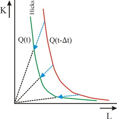
Figure 3: Hicks neutral isoquants
Until now the development of Q in time has been ignored. However, this column wants to study the dynamics of the technical progress. New techniques will raise the productivity of the production factors. Thus the time must be included in the production function, which then becomes Q(t) = F(q, t). In order to limit the complexity of the theory, henceforth merely two production factors will be considered, namely the labour L and a capital good K. The famous economist J.R. Hicks has proposed to model the technical progress by means of production functions of the form
(5) Q(t) = A(t) × F(K, L)
The factor A(t) is a measure of the level of the technology at the time t, and is called the total factor productivity. The technical progress, which is expressed by the formula 5, is called Hicks neutral. Note that although the quantities of the production factors K and L can change with time, nevertheless their functional behaviour F(K, L) remains conserved. This probably explains the term "neutral" for this form of progress. One can define A(0) = 1 without any loss of generality. Since progress implies an increasing productivity, one must have A(t) > 1 for t>0.
The technical development under Hicks-neutral conditions can be illustrated by means of the isoquant Q(t) = Q(0) = Q0. For, in a situation with a constant Q0 and a rising productivity the quantities of K and L can decrease. On the isoquant the increase of A(t) is compensated by the fall of K and L. When the function F(K, L) is linear-homogeneous, like the neoclassical paradigm assumes, then one has Q0 = F(K × A(t), L × A(t)). When at t=0 the starting point is (K, L) on the isoquant with capital intensity k=K/L, then at a later time t>0 that point will move towards the origin without changing k. The figure 3 illustrates this time behaviour of isoquants under Hicks-neutral conditions9.
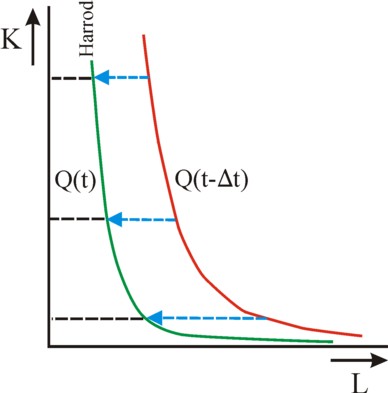
Figure 4: Harrod neutral isoquants
The famous economist R.F. Harrod was not particularly satisfied by the formula 5 for the technical development, because he foresees problem in the empirical determination of the quantity K of the capital good. He believes that it is easier to compare situations of equal K, and to study exclusively the improvement of the labour productivity Q/L. This leads to production functions of the form
(6) Q(t) = F(K, A(t) × L)
The technical progress, which is described by the formula 6, is called Harrod neutral. Also here the functional behaviour remains conserved, provided that the calculations use F(K, Λ(t)) and Λ(t) = A(t) × L. Suppose for convenience again that A(0) = 1, then one has Λ(0) = L. Λ increases for t>0, not because the working-hours are increased, but because the productivity of the quantity L of labour rises10. Also under Harrod-neutral condition the technical development can be illustrated by means of the isoquant Q(t) = Q(0) = Q0. The increase of A(t) must be compensated on the isoquant by a proportional decrease of L. When at t=0 the starting point is (K, L) on the isoquant with capital coefficient κ=K/Q, then at a later time t>0 that point will move to the K-axis without changing κ. The figure 4 illustrates this time behaviour of isoquants under Harrod-neutral conditions11.
Finally this micro-economic argument must be completed with a much-used mathematical formula for the production function. The names of the North-Americans Cobb and Douglas are attached to this function, because they have made her popular. She is12
(7) Q = A × Kβ × Lα
Since this function is applied mainly to static situations, the variable t is omitted. The constants α and β are positive. As always, K and L are complete substitutes for each other. The formula 7 is very convenient for practical applications. For instance, the formula 7 can be rewritten as K = (Q / A)1/β / Lα/β, so that apparently the isoquants behave as hyperbolas in the (L, K) plane.
The reader can check easily that the Cobb-Douglas functions is homogeneous of degree α+β. Therefore in the popular linear-homogeneous case β equals 1−α. And the marginal productivities are ∂Q / ∂K = β × Q/K and ∂Q / ∂L = α × Q/L. When α and β are less than 1, which is a common assumption, then the marginal productivity of a factor is apparently less than the average productivity (namely, Q/K and Q/L). It follows immediately that the marginal productivity of a factor decreases, according as he is more abundantly present. According to the formula 4 another interesting property of the Cobb-Douglas function is, that the marginal substitution rate MSVLK equals k × α/β. MSVLK remains unaltered along a line of constant capital intensity.
The macro-economic production function
Cobb and Douglas became famous, because they have applied the function of the formula 7 at the macro level. The nation-state is presented as an enormous enterprise, as it were. It is obvious, that there are large practical problems attached to this approach13. For, it is an impossible task to aggregate all production factors of the state into a single production function. They are too numerous. Perhaps the loyal reader will object, that at least fot the case of complementary production factors the theory of Sraffa can be applied. But even those simple formulas are only applied in situations with separate economic sectors, and not at the level of the separate enterprises.
However, the studies at the sectoral level must necessarily already use aggregation. The separate capital goods are collected in a limited number of categories. The aggregation of heterogeneous goods is only possible by means of their monetary value. In the Cobb-Douglas function this happens in a rigorous manner, because only a single capital factor K remains. The same approach is used in the well-known growth model of the economist R.M. Solow. However, problems surface when values are used in the production functions. For, the production functions represent a certain technique. As soon as values are included, then the social variables such as the wage level and the interest rate will also affect the result.
At the micro level, for the separate enterprise, the production prices and the factor prices are given, at least as long as the market is ruled by perfect competition. But this assumption is no longer valid at the aggregated macro level, because there the prices are mutually coupled. For instance, as soon as production factors are substituted, the prices will change, as well as the resulting aggregated values. Thus the total product Q can change in value, although perhaps the material itself remains the same. This results in apparently strange phenomena, certainly for the neoclassical economists, such as the reswitching of previously rejected production techniques.
The difference between the micro and macro level can also be illustrated well by means of the relation between the marginal productivities and the factor prices. The formula 1 shows that at the micro level the entrepreneur tries to make his yield as large as possible, and to minimize his costs. His method is shown in a graphical manner in the figure 2. The production costs are TC = K × pK + L × pL. This is the green straight line in the (L, K) plane, and is called the budget line. In the same plane the isoquants are drawn, which belong to his production function f(K, L).
Now the entrepreneur tries to produce at the highest possible isoquant, that is within his reach. That reach is limited by the sum TC, which he owns. The optimum of the entrepreneur is the point of the budget line, that just touches the isoquant. A higher isoquant is beyond his range. In the optimum the slope of the budget line (which is -pL/pK) is exactly equal to the slope of the isoquant (which is MSVLK, and thus satisfies the formula 4). This leads to the formula14
(8) (∂Q / ∂L) / pL = 1/π = (∂Q / ∂K) / pK
In the formula 8 π is a constant, whose value can be determined by a simple argument. Namely, in most circumstances the marginal productivity ∂Q / ∂L will be a positive but nonetheless falling function of L 15. An entrepreneur continues to hire workers until the value of their marginal productivity has fallen to the wage level. That endpoint satisfies pL = ∂(p × Q) / ∂L = p × ∂Q / ∂L. This is precisely the formula 8, with π=p. A similar argument can be made for the factor capital.
Does the relation pn = p × ∂Q / ∂qn also hold at the macro level? Even nowadays some introductory textbooks state that this is true16. But it is wrong, because at the macro level the product prices p and the factor prices pn are themselves variables, and they depend on Q and qn. The micro-economical argument can not be copied in macro-economics.
In conclusion, the reader is once more reminded that this critique on macro-economical applications also holds for the growth model of Solow. For, that model also aggregrates the physical products into monetary sums, namely the factor capital K(t) and the nett product N(t). The values of all those monetary sums will vary, according as different production techniques are used. In fact the production function of Solow does not represent a technique any more17.
- A large number of textbooks is consulted for this column, mostly of the introductory type. A very complete book, and in the Dutch language, is Micro-economie (1996, Stenfert Kroese) by F.J. Dietz, W.J.M. Heijman and E.P. Kroese. This publication compares well with foreign books, and moreover gives information about the Dutch economy and about the publications of Dutch economists. A minor objection is that the authors remain rather silent about the theoretical deficits of the common neoclassical paradigm. For a critical evaluation of the theory the reader can consult Volkswirtschaftslehre (2003, Oldenbourg Wissenschafts-verlag) by M. Heine and H. Herr. Less advanced but easily accessible is Mikroökonomische Theorie (2011, UVK Verlagsgesellschaft mbH) by W. Hoyer and W. Eibner. Rather succinct but yet interesting is Microéconomie (1991, Presses Universitaires de France) by F. Etner. Besides, your columnist has consulted the relevant chapters in the advanced book Economie en technische ontwikkeling (1973, H.E. Stenfert Kroese B.V.) by A. Heertje.
The column argues along the lines of the experimental reader Vooruitgang der economische wetenschap (2011, Uitgeverij E. de Bibelude) by E.A. Bakkum. Most of the figures stem from this reader. It is worth mentioning, that at the time the reader has been offered for free to several student associations. This elicited just a single reaction, namely that the members had more important pursuits than correcting these texts. This furthers modesty. Apparently the average student does not find his happiness in professional knowledge. (back)
- Note that the production functions satisfy cardinality. That is to say, the evaluation of the functions leads to a quantitative value, so to a real number. Furthermore, note that the output of one enterprise can be used as the input for another enterprise. An enterprise can even use a part of her own production Q as the production factor in her own production function. For the sake of convenience most introductory textbooks assume, that the production is a continuous process, and not incidental or periodical. (back)
- Here business economics must be consulted. Or the literature, for instance the play Glück auf! by Herman Heijermans: (Director of the mine): Since we are associated with the syndicate. we must consult the syndicate. (Manager of the mine): Mister chairman, I ask for the third time to vote. Just now the honoured questioner ignored that we can only make a profit, as long as the local movement becomes general. In the struggle for power ... (Shareholder): Yes, yes but, but, provoking a strike, while the stocks are rather large at the start of the winter ... Mister chairman, I defend the interests of the small shareholders, who have invested their saving in our enterprise - I say, that we had in ninety-seven, that the mine degraded gravely during the strike of six weeks ... (back)
- The Leninist economists will not support this. For, when an entrepreneur maximizes his profit, he will push his less skilled competitors from the market. Therefore, it would be advantageous for society as a whole, when the successful entrepreneur voluntarily limits his market share, at least for the time being, until the equipment of his competitors has been scrapped. The sociologist Schumpeter used to say, that in capitalism the creative destruction rules. (back)
- For, f(q) × p − q · p = q1×p × { f(q) / q1 − (q/q1) · p/p } = q1×p × { q1γ-1 × f(q / q1) − (q/q1) · p/p }. The multiplication with p naturally does not affect the maximization, so that it can be omitted.
The vector q/q1 has as its elements qn/q1, and these are the factor-intensities. These, in combination with the term q1/Q, can be used to derive the production coefficients, which are known from the Leontief-model. The vector p/p has as its elements pn/p, and that is the price ratio of the production factor n and of the product. (back)
- Namely, suppose that the technique is given. Then all qn/q1 are fixed. In that situation the maximization of the formula 3 implies that one must have ∂(q1 × Ψ(q / q1)) / ∂q1 = 0. Therefore one has Ψ(q / q1) = 0, which had to be proven.
Since in this argument q1 plays the role of a scaling factor, the marginal productivity ∂Q/∂q1 is also the so-called marginal return to scale. Note also, that Ψ in this situation represents the difference between the yield and the production costs. Therefore Ψ=0 implies, that the yield is distributed competely over the production factors, as their incomes. There is no residual, as a profit for the entrepreneurs. (back)
- All neoricardian models, that use the theory of Sraffa, are of the Leontief type. The interested reader is encouraged to consult on this portal the many columns, which have been published about this theme. (back)
- For, along the isoquant one has dQ = 0. That is to say, one has Σn=1N dqn × ∂Q /∂qn = 0. Consider a plane (qν, qμ) with dqn=0 for all n except ν and μ. Then one has dqμ / dqν = - (∂Q / ∂qν) / (∂Q / ∂qμ). And the term in the left-hand member of the equation is precisely MSVνμ. This completes the proof. (back)
- The figure is drawn for the isoquant 9 = K¼ × L¾. It is assumed that during a time Δt the factor productivy increases with 1.5 (that is to say, 50% growth). (back)
- The Flamish play writer Walter van den Broeck depicts the technical development in Tien jaar later: 't Jaar 10: (Albert): It is the same everywhere. They all close. (Jan): Not the Vieille Montagne, I tell you. Not the Vieille Montagne! (Luc): Do you still not understand? First they have sold the cité, turned everybody into small, scared owners. Then they have closed one department after another. It is true, you were a peeler. Why did you stop? Because you were useless. In those automated super-halls, today they peel more there than before in all halls together. These days even the artisans peel one in five weeks. I tell you that the Vieille Montagne will close and you can say what you want. (Jan): And all those millions of the state then? Why are they supplied? (Luc): To speed up the automation. To lay off still more workers. (back)
- This figure is also drawn for the isoquant 9 = K¼ × L¾. It is assumed that during the time Δt the productivity of labour increases with 2.25 (that is to say, 125% growth). Since the Harrod neutral technical development merely affects the factor labour, the shift of the isoquant is still close to the shift for the Hicks neutral technical development of the figure 3. (back)
- The multi-dimensional equivalent of the Cobb-Douglas functie is Q = A × Πn=1N qnαn. In this formula Π is the mathematical expression for the multiplication of the N terms qnαn. Most of the properties of the Cobb-Douglas function can be easily extended to the case of its N-dimensional equivalent. (back)
- There even exists a Dutch book about this theme, namely Economie en technische ontwikkeling (1973, H.E. Stenfert Kroese B.V.) by the economist A. Heertje. It is a difficult book, which summarizes the then topical scientific literature about this theme. The author may have overestimated the size of his Dutch audience somewhat. Your columnist acquired the book at the second-hand bookshop De Slegte, just before it went bankrupt. (back)
- First of all, note that the MSVLK is defined as a positive value. Therefore also the slope pL/pK must be a positive number. Then one has (∂Q / ∂L) / (∂Q / ∂K) = pL / pK. Move all quantities of a production factor to the same side of the equation, then it follows that (∂Q / ∂L) / pL = (∂Q / ∂K) / pK. It is of course allowed to designate the left-hand and right-hand side as 1/π. (back)
- This can also be formulated as follows. One has dQ(K, L) = ∂Q/∂K × dK + ∂Q/∂L × dL. Consider the change along a path with a constant capital intensity k=K/L. That is to say, K and L scale in the same way. Use L as the scaling paramter, then one has dQ/dL = k × ∂Q/∂K + ∂Q/∂L. it follows that (dQ/dL) / (Q/L) = (∂Q/∂K) / (Q/K) + (∂Q/∂L) / (Q/L). Expressed in words: the elasticity of the scales equals the sum of the separate production elasticities of the factors. The elasticity of the scales can exceed 1, for instance for above-linear homogeneous production functions. But usually she will deviate so little form 1, that the production elasticities of the separate factors are less than 1. In the formula for the general case this statement is ∂Q/∂qn < Q/qn, for the variation of qn in an otherwise unchanged situation. The marginal increase is less than the average increase. Therefore the growth of the function Q(qn) apparently diminishes, according as qn increase. The slope of Q approaches zero.
For the sake of completeness here a remark must be made, which may somewhat confuse the reader. The statement ∂Q/∂qn < Q/qn is valid only as long as only the factor qn changes. In the described formula for the differential dQ this is by definition true. But when at the same time also the quantities of other production factors qm (with m unequal to n) are changed, such as in a general increase of scale, then this obviously also affects Q. The marginal productivity ∂Q/∂qn "benefits" from the other rising marginal productivities ∂Q/∂qm. So in a general increase of scale ∂Q/∂qn > Q/qn is possible. This situation occurs in particular, when increasing returns to scale are present. The entrepreneur can no longer reward the factors according to pn = p × ∂Q / ∂qn, because then the factor is paid according to his last added, most productive unit. In other words, the formula is only valid as long as the marginal productivity really decreases with a rising qn. (back)
- See for instance p.51 in Macroeconomics (2000, Worth Publishers) by N.G. Mankiw. There Mankiw makes the step from a single enterprise to the national economy, without excuse or or stings of conscience. Apparently prejudice and mental inertness last long. There are even Dutch universities, that teach with the textbooks of Mankiw. This merits the attention of future students ... (Yes, your columnist is indignant) (back)
- On p.180 of Economie en technische ontwikkeling Heertje states that Solow simply assumes the macro-economic production function, that is to say, as an hypothesis. But then it is not clear, what the substitution between K and L actually means. (back)