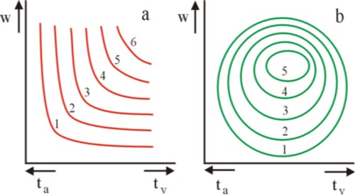
Figure 1: iso-utility mapas: (a) convex; (b) utility mountain
The neoclassical theory assumes that the wage and the leisure time are more or less substitutes. This column explains, that according to R. Layard the substitution is not quite rational, due to human rivalry and habituation. Furthermore, a model of collective bargaining is presented, with the wage and leisure time as stakes. It reminds of the work of Sam de Wolff. Finally, it is discussed that in happiness economics, Van Praag analyzes the human preferences by means of the probit method.
In a previous column it is described how the neoclassical theory models the supply of labour on the labour market. The level of the wage w and the leisure time tv can be exchanged, at least to a certain extent. Those who prefer more leisure time, can work less, which translates into a lower income. Thus each worker can decide for himself, which combination of tv and w is most desirable. The personal preference is described mathematically by the utility function u(tv, w). Suppose that the worker disposes of a total time T, to be used at will. That is to say, T has been stripped of the absolutely necessary activities such as a minimal time for rest and meals. Then the leisure time equals tv = T − ta, where ta represents the labour time.
Furthermore, it must be remembered, that the income w merely is a secondary variable. The workers are really interested in their consumption c. Therefore in the present column the variable c will often be used, with the implicit assumption that c = w. Besides, it is assumed, that merely one consumer good is supplied. For, as soon as various consumer goods are available, a change in income will have unpredictable effects on the prices of those goods. The price changes affect the consumer behaviour, including the choice of leisure time. Therefore in a multi-goods economy the leisure time tv is as unpredictable as the prices. Besides this fundamental limitation, the neoclassical model of the labour market suffers from various other shortcomings. For more information, the interested reader is referred to the mentioned column. The model must not be taken too seriously, because it is an abstraction. As such it helps to frame the arguments.
The mentioned column presents a sketch of the indifference field or iso-utility field of u(tv, c). According as the theory gets more abstract and uses more mathematical formulas, she can derive more relations. Unfortunately, the theory also becomes less realistic. Thus it is often assumed, that the preferences are desirable and convex1. The assumption of a desirable preference implies, that an increase of the quantity of the consumer good always raises the utility. The assumption of a convex preference refers to the willingness to exchange two consumer goods. Consider the example u(tv, c), as in the figure 1a. On an iso-utility curve u is constant, in other words, the worker can exchange (or substitute) tv and c without changing his utility. In the mentioned previous column it is shown, that the rate of substitution equals MRS = ∂c/∂tv = -(∂u/∂tv) / (∂u/∂c). Now the hallmark of the convex preference is, that MRS decreases in absolute value according as tv increases.
The convexity can be made credible as follows. Due to the desirable preference, ∂u/∂tv and ∂u/∂c are both positive. Therefore the MRS is negative, that is to say, more leisure time leads to a reduced consumption. According as the consumption becomes more scarce, the worker is less willing to give up an extra unit of consumer good. He wants much extra leisure time as a compensation. And that fact lowers his MRS. Apparently, in case of convexity the absolute value of the MRS is a falling function of tv. The MRS is called marginal, because it refers to a marginal change. The convex preference can be explained as a leaning towards diversity. The worker does not like extremes, but wants to balance the satisfaction of all his needs.
At first sight the assumptions of desirable and convex preferences seem reasonable. However, already in 1854 Hermann H. Gossen, the founder of the neoclassical theory, has criticized these two abstractions. Namely, when somebody acquires too much of a certain consumer good, the utility changes into a burden. Then the so-called marginal utility ∂u/∂c becomes negative. This property also holds for the leisure time, because workers do derive pleasure from their work, at least as long as the working time ta remains within limits. Thus in a previous column it is concluded that in reality the iso-utility curves are ellipses. In fact the indifference field is a utility mountain, as shown in the figure 1b.
The utility mountain can actually be found in the arguments of the Dutch economist Sam de Wolff, who adopts the main ideas of Gossen. This is apparent from the column about the labour theory of value of De Wolff. There De Wolff assumes, that the labour productivity is constant. Then the utility function obtains the form2
(1) u(tv, c) = γ − α1 × (tv − α2)² − β1 × (c − β2)²
The formula 1 shows, that in case of positive constants the iso-utility curves have the form of ellipses in the (tv, c) plane. The utility mountain reaches its top u=γ at (α2, β2). Here it is immediately noted, that the model of De Wolff is a so-called Robinsonade, which represents the situation of an isolated individual. That situation is evidently exceptional, and not representative of the economy. Nevertheless, his model is interesting, because it illustrates well the complexity of preferences. According to the formula 1 the iso-utility curves are no longer convex, when one has tv ≥ α2, or c ≥ β2. In those cases the marginal rate of substitution MRS behaves in an extraordinary manner. Besides, on the lower iso-utility curves the situation may occur, that one has tv=0 or c=0. In such a situation the scarcity of a good is never so pressing, that the MRS approaches infinity or zero in absolute value. Then the worker is willing to prefer an extreme.
In short, it is perilous to abstract in the domain of human preferences. After this warning, next two models of the labour market will be discussed, that significantly simplify the utility function u(tv, c). Namely, they assume that one has3
(2) u(tv, c) = tv1 − δ × cδ
In the formula 2, δ is a constant with values between 0 and 1. It measures the materialism of the worker. For, at δ=1 he is only interested in consumption. This type of function is called a Cobb-Douglas function. The formula 2 represents a utility, that is desirable. For, ∂u/∂c = δ×u / c and ∂u/∂tv = (1 − δ)×u / tv. Moreover, that utility exhibits a convex behaviour, because on the iso-utility curve one has MRS = -(c/tv) × (1 − δ)/δ. For an increasing tv this rate of substitution will fall in absolute value. Thus the Cobb-Douglas function represents a theoretically practical utility function.
The present paragraph is based on the contribution of the economist R. Layard in the book Economics and happiness4. The text of Layard concerns happiness economics. In his contribution he studies two forms of irrational behaviour in the labour market, namely rivalry and adaptation. They are both a consequence of workers, comparing their incomes with those of people in their surroundings, the so-called reference group. First, consider rivalry, which is incited by the differences in income. A worker, who earns relatively less than his reference group, becomes dissatisfied and therefore will be inclined to work harder.
Layard judges negatively with regard to the impulse of rivalry. Namely, according as the displeased worker improves his income, the other people in his reference group will become more dissatisfied in their turn. Thus they will also be incited to work harder. When these people would realize, that they are incited by their mutual rivalry, then they would all prefer to work less, and yet remain about equally satisfied. Layard wants to analyze this phenomenon of irrational behaviour, and therefore develops a model based on the utility formula 2.
Layard believes that because of the influence of rivalry, it is not the consumption c of the worker, that must be inserted in the formula 2, but his consumption with respect to the average consumption level cgem in the group of the worker. To be precise, he replaces the formule 2 by
(3) u(tv, c) = tv1 − δ × (c − β×cgem)δ
The constant β in the formula 3 is a positive weighing factor of the average consumption level, which expresses the degree of rivalry. The formula 3 does not have a theoretical justification, but is purely empirical. The rivalry removes a part of the consumer satisfaction, and more according as β×cgem/c is larger. The consumption of the worker is given by c = w×ta = w × (T − tv). Now the worker will choose the time tv, that maximizes his utility. In the utility maximum one must have ∂u/∂tv = 0. It is clear from the formula 3, that the maximum is obtained for5
(4) tv = (1 − δ) × (T − β × cgem / w)
That is to say, when β=0 (no rivalry), then the maximum is at ta = δ×T. However, when β>0, and thus rivalry is present, then the workers reduces his leisure time. His working-hours increase with (1 − δ) × β × cgem/w. It has just been concluded, that in this manner his group becomes less satisfied. Suppose that the total group of the worker consists of N people. Then each extra unit of consumption of the worker increases the average standard of living cgem with 1/N. In this manner each of the other group members loses (1/N) × ∂u/∂cgem of his satisfaction. When all the lost satisfaction is aggregated in a cardinal manner, then the group as a whole loses ∂u/∂cgem of satisfaction.

Another irrational behaviour is the adaptation or habituation with respect to an amelioration of the income. This phenomenon is caused by the human inclination to change one's reference group, according as one earns more. At the time the Dutch economist B. van Praag has named this phenomenon the preference drift. People are in advance poorly conscious of the fact, that after an improvement of their income they will adapt their needs. Therefore they attach a priori more value to the wage rise than is actually justified. This also is an unnecessary incitation to work hard.
Layard analyzes the habituation by dividing the life of the worker in periods π. He believes that in a dynamic situation the worker does not optimize his utility u(π) for each period, but the aggregated utilities during his lifetime. Besides, people prefer to obtain their utility as soon as possible, with the consequence that the utilities of periods in the distant future must be depreciated with respect to the present. Suppose that the worker from now onwards will live for another ω periods, then his total utility of life becomes U = Σπ=0ω u(π) / (1 + r)π. The factor r is the discount rate of the utility for the concerned worker. For the sake of convenience Layard defines R = 1/(1+r). Now the worker optimizes his utility of life U by calculating all periodic marginal utilities ∂U/∂tv(π).
To be honest, the approach of Layard in analyzing the preference drift does not yield many useful insights. In fact, it raises several questions, so that the reader may do wise to skip to the next paragraph. Nevertheless, yet his arguments are presented here for fanatics. In the most general case the wage in the period π equals w(π). It is a source for consumption with a size of w(π) × (T − tv(π)). Besides, the worker can save a part of his income, which can be spent during a next period. This decouples the wage and the consumption somewhat. The change of the consumption at the start of a period π can be defined as Δc(π) = c(π) − c(π-1). Due to the adaptation the utility of a positive Δ will be partially lost. In that way Layard derives the utility function6
(5) u(tv(π), c(π), c(π-1)) = tv1 − δ × (c(π) − γ×c(π-1))δ
In the formula 5, γ is an empirical constant. It is obvious that this formula is also more empirical than theoretical, just like the formula 4, and incidentally like the Cobb-Douglas relation itself. Now, thanks to the formula 5 Layard can calculate ∂U/∂tv(π). The procedure is as follows. Each tv(π) appears twice in U, namely as the start of the period, and as its end. Therefore a differentiation with respect to tv(π) yields merely two non-zero terms, where the highest one is yet depreciated with R. Nevertheless, the resulting expression is still too complex7. Therefore, now Layard assumes, that there are no savings, so that the relation c = w×ta holds again. Moreover, he assumes that all other variables remain unchanged. That is to say, c and tv are constant for all periods π. Then one has u = tv1 − δ × ((1−γ) × c)δ, also independent of π. After some rewriting Layard finds as the result for the optimal tv
(6) tv = (1 − γ) × (1 − δ) × T / ((1 − γ×R) × δ + (1 − γ) × (1 − δ))
When one has γ=0, then there is no preference drift, so that the now familiar relation tv = (1 − δ) × T holds. The effect of a positive γ is illustrated well by first writing the expression tv = (1 − δ) × T / (δ × (1 − γ×R) / (1 − γ) + 1 − δ). For, R is less than 1, so that here the term (1 − γ×R) / (1 − γ) is larger than 1. The consequence is that the denominator is larger than 1, and finally tv is less than (1 − δ) × T. Thus it turns out that the adaptation indeed incites to work longer. One may wonder, whether this analysis is worth the trouble, considering this meagre result. Anyway, it did not cost your columnist the time, that Layard undoubtedly had to invest in it.
Layard uses the formulas 4 and 6 for calculating the effects of rivalry and of adaptation with several numerical examples. Besides, he calculates the size of the tax rate on consumption, that is needed to compensate for the incitations of rivalry and adaptation. Layard believes that such a tax is relevant, because he fears that otherwise the work load will become too high and the society will become too materialistic. In that sense he is truly a congenial of the politician Femke Halsema. However, your columnist is not convinced. For, rivalry and adaptation are typical human properties, which certainly have positive effects for the individual and the society. It would be wrong to merely pursue the satisfaction and utility as the ultimate human goal.
In a previous column two models have already been presented for the analysis of collective bargaining. The present paragraph adds a third model, where the bargaining concerns both the wage w and the working-hours ta = T − tv. The model is again copied from the book Labor economics by P. Cahuc and A. Zylberberg8. It fits well in the present colmn, because it chooses the formula 2 as the utility function of a union member, with c=w. The enterprise naturally has the aim to maximize its profit Π(ta, w, L) = Q(ta, L) − w×L. The enterprise keeps the right to manage, that is to say, the control of the number L of workers employed.
A worker will obviously produce more according as he works for more hours. It seems reasonable to assume that the labour productivity behaves as
(7) ap(ta) = ap(1) × taβ
In the formula 7, ap(1) is the labour productivity during the first working-hour. The parameter β is a constant, which represents the elasticity of the productivity with respect to the working-hours. It seems logical to choose β between 0 and 1. This implies that the increase of ap with time has the tendency to level off. The marginal product of the working-hours decreases, because the worker becomes somewhat tired. In mathematical form this is ∂ap/∂ta = β × ap/ta > 0 and ∂²ap/∂ta² = β × (β-1) × ap/ta² < 0.
Next the behaviour of the production function Q(ta, L) must be determined. The production is not simply equal to ap×L, because the enterprise merely disposes of a limited quantity of capital goods. According as more workers are hired, the production per unit of capital will decrease. The marginal product of the factor labour diminishes. In the model a choice is made for the production function
(8) Q(ta, L) = (ap(ta) × L)α / α
In the formula 8, α is a positive constant with a value between 0 and 1. Thus the formula can be interpreted as the labour part of a Cobb-Douglas production function.
The formula 8 can be inserted in the profit formula. Next the profit can be maximized by chosing L in such a manner that the condition ∂Π/∂L = 0 is satisfied. Then the optimal solution is
(9) L(ta, w) = (ap(ta)α / w)1/(1-α)
Finally, thanks to the formulas 8 and 9 the optimal profit function of the enterprise can be calculated, at least for L,
(10) Π(ta, w) = ((1-α)/α) × (ap(ta) / w)α/(1-α)
The goal of the trade union movement must be formulated as well. Suppose that all union members have about the same preferences. An individual income y gives to each of them a utility u(y). Suppose that the union has N members. In other words, a fraction λ=L/N of the members acquires a job at the enterprise. The remainder of the members is unemployed, and obtains a benefit x from the state. Obviously x is less than w. Then the satisfaction of the union members can be represented by
(11a) U(tv, w) = λ × u(tv, w) + (1 − λ) × u(T, x) that is to say
(11b) N × U(tv, w) = L × (u(tv, w) − u(T, x)) + N × u(T, x)

For the sake of convenience it is assumed, that during the bargaining the union attempts to make the total utility U (or N×U) of its members maximal. The members are certain to obtain the benefit, so that the maximization concerns merely the first term in the right-hand side of the formula 11b. Thus it seems reasonable to represent the collective bargaining by the expression
(12) choose from all tv and w the ones, that maximize the variable ψ = Π1-γ × (L × (u(tv, w) − u(T, x)))γ
In the formula 12, γ is a measure of the power of the trade union. For, when γ=0, then merely the profit is relevant, and the preference of the union does not count. And when γ=1, then the profit is unimportant. For the intermediate values of γ the interests of the enterprise and the union are both taken into account.
The problem can also be formulated as follows: in the optimum one must have ∂ψ/∂tv = 0 and ∂ψ/∂w = 0. The outcome is called the general Nash solution, in honour of the mathematician John Nash. The two differentiations can be worked by inserting the formulas 2, 7, 9 and 10 in the ψ of the formula 12. Next tv can be calculated from the equations ∂ψ/∂tv = 0 and ∂ψ/∂w = 0. The result is9
(13) tv = (1 − δ) × (γ + α × (1 − γ)) × T / (α×β×δ + (1 − δ) × (γ + α × (1 − γ)))
The reader may again recognize in the formula 13 the term (1 − δ) × T, which represents the materialism of the worker. Furthermore, note that the numerator contains a term γ × (1 − α). Apparently the leisure time increases, according as the union disposes of more power. In times of high unemployment the trade union is less powerful, and then the enterprise will apparently dictate long working-hours.
Finally, it must be remembered that Sam de Wolff, the name-giver of the Gazette, has modelled the collective bargaining already eighty years ago. His model is described in a previous column. De Wolff characterizes the power of the union as the degree, in which she can extort the nett-lust of the workers (the constant κ in the column). During the collective bargaining the union uses κ as an iso-utility curve in the (tv, w) field. In other words, the entrepreneur is free to exchange wage and leisure time, as long as the nett-lust κ is maintained. Thus according to De Wolff the trade union bargains with regard to both the wages and the working-hours. It is striking, that the same freedom of substitution is present in the formula 2.
Furthermore, the model of De Wolff describes the consequences of a reduction of the power of the union, that is to say, a decreasing κ. In that situation the entrepreneur will increase his profit by lowering the wage, and increasing the working-hours. In the model the entrepreneurs keep the free right of management, so that they can determine L by themselves. So, just like the presented model, De Wolff assumes a structural unemployment. According to him that unemployment is voluntary, which is a rather curious idea for an orthodox marxist. A part of the workers simply believes that the wage is not a sufficient reward for the job, and resigns. Nevertheless, the model is De Wolff has its merits, also because of its simplicity.
Until recently, the empirical information about substitution of leisure time for wage mainly had a qualitative character. However, ten years ago the economists Bernard van Praag and Ada Ferrer-i-Carbonell have in their book Happiness economics made a thorough statistical analysis of human preferences, including the needs in a business environment10. The present paragraph will describe their results, as far as they concern the substitution of leisure time for wage. The empirical data originate from population surveys in West-Germany, East-Germany and England. In these surveys various types of factual data about citizens have been collected, such as their income, age, sex, relations, health, hobby's, housing, etcetera. Besides they have been interviewed, among others about their satisfaction with various aspects of their life.
Such a data set is very suited for a statistical analysis with the probit method. And this has indeed been done by Van Praag and Ferrer-i-Carbonell. Thus, for instance the citizen k was asked to give marks concerning his satisfaction with his job. This mark u(k) can be interpreted as the utility of the citizen.. Next, u(k) can be correlated with the actual situation of the citizen k by means of a statistical fit. For this purpose, the probit method employs an equation of the form
(14) u(k) = α1 × ln(w(k)) + α2 × ln(ta(k)) + α3 × ln(c(k)) + α4 × ln(lt(k)) + α5 × g(k) + α6 × ln(f(k)) + ...
In the formula 14, w, ta and c have the usual meaning. However, here w must be interpreted as the yearly wage, not as the hourly wage. And c can exceed w, for instance when someone also receives interest as an income from capital. Furthermore, the symbol lt refers to the age of citizen k, g denotes the sex, and f is the number of members in his or her household. The probit method estimates the empirical values of the coefficients αn (with n = 1, 2, 3, 4, ...) by optimally approximating the left-hand side of the formula 14 by the right-hand side, for all citizens k in the survey.

The formula 14 has the agreeable property that she has the same form as the formula 2. For, the formula 2 can be transformed in a logarithm, so that one has v = ln(u) = (1 − δ) × ln(tv) + δ × ln(c). Therefore all formulas in this column can be applied fairly simply to the formula 14. For instance, an iso-utility curve u = constant can be considered, and its marginal rate of substitution can be calculated for two variables. Thus one has for the wage and leisure time MRS = ∂w/∂tv = -∂w/∂ta = (∂u/∂ta) / (∂u/∂w) = (α2/α1) × w/ta. As an alternative the so-called elasticity η, which is connected to the MRS, can also be calculated. Whereas the MRS expresses the absolute changes of two variables, the elasticity expresses the relative changes. She is defined as η(tv, w) = MSV(tv, w) × tv/w. Or, if desired, as η(tv, w) = (∂w/w) / (∂tv/tv). In the same manner as for the pair (tv, w), the MRS and elasticity can be calculated for various pairs of variables. For instance, in the present discussion it is logical to calculate η(ta, w) = α2/α1.
An interesting result of the probit method can be found on p.60 in Happiness quantified. There the satisfaction u with the job is analyzed for the English workers. The probit method yields α1 = 0.416 and α2 = -0.031. The minus sign obviously expresses, that long working-hours are experienced as a burden. It follows that MRS(ta, w) = 0.075 × w/ta, and that η(ta, w) = 0.075. This shows that long working-hours can in principle be compensated by a higher wage. Unfortunately, Van Praag and Ferrer-i-Carbonell do not mention anywhere in their book the units that are used for the variables w, c, ta etcetera. Therefore these statistical data are only usable for qualitative conclusions, and for relative comparisons, where the units cancel.
Interesting is also the analysis on p.95 in Happiness quantified, where the satisfaction u with the labour income is studied, for the same group of English workers. Here one has α1 = 0.165 an dα2 = -0.076. However, the two authors have also added a term α7×ta to the formula 14, thus without logarithm. Here it is found that α7 = -0.214. Therefore one has MRS(ta, w) = -(α2/ta + α7) / (α1/w) = 0.43 × w/ta + 1.3×w. This also changes the elasticity, namely η(ta, w) = 0.43 + 1.3×ta. In this case the elasticity is not constant, but she increases for the longer working-hours. Indeed it is by no means evident, that an elasticity must be constant. Your columnist can not explain, why this elasticity behaves different from the one in the immediately preceding text.
The described empirical results strenghten the hope, that the probit method is quite versatile. Unfortunately, the results are sometimes less convincing. For instance, p.58 in Happiness quantified shows the analysis for the German workers, and there it turns out that the job satisfaction does not correlate with the working-hours ta, at least not in a statistically significant manner11. In view of all the theoretical ideas in this column and the results of the English study this empirical find is surprising. The cause must be searched in the huge practical and methodological problems, which must be overcome for measuring the statistical data in a reasonably reliable manner. These obstacles emerge in particular, because the sought effects are actually rather small. It is true that an average man with characteristic properties can be identified, but the spread around this average is manifold, multifarious and often considerable.
Therefore it is understandable that Van Praag and Ferrer-i-Carbonell have forgone an explanation of the many significant differences between the German and English measurements of human preferences. For the moment, doubts can even be raised about the practical applicability of such empirical studies. When in this early phase the sociological and economic measurements of the human preferences are used to justify the political policy, it invites manipulations and pseudo-science by charlatans. Nevertheless, your columnist believes, that Van Praag points in the right direction for future attempts to model the human behaviour in a quantitative sense12.