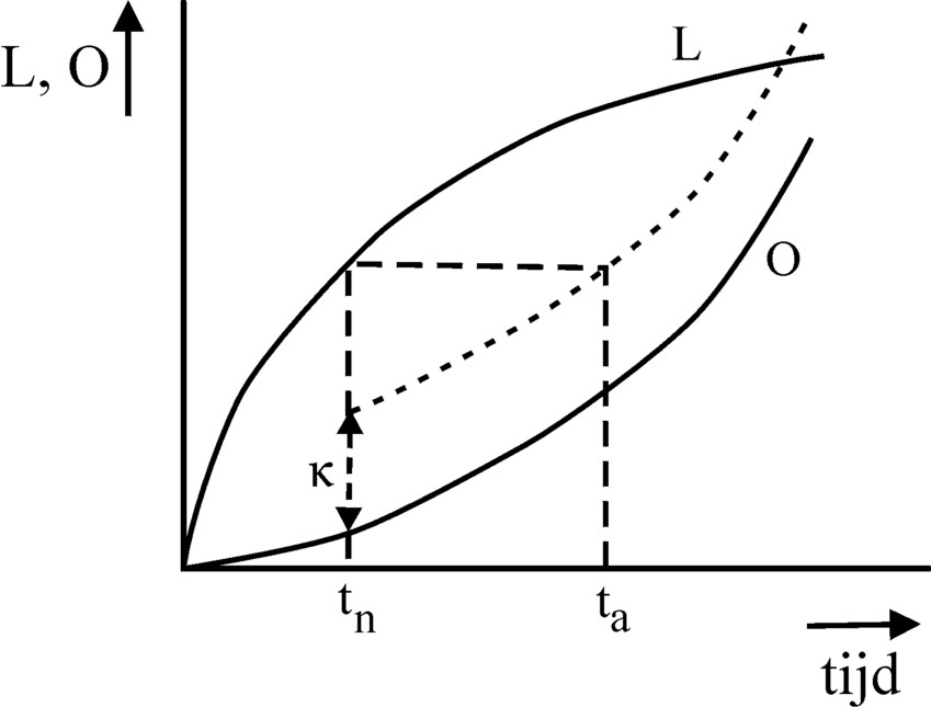
Figure 1: (tn, ta) pairs for L and O curves
One of the most original parts in the main work Het Economisch Getij of Sam de Wolff is the paragraph, where he describes the driving forces behind the size of the national product1. In fact the size of the production is not the main theme of the research of De Wolff, for this focuses on the business cycles. However, De Wolff thinks that the conjuncture can only be understood in conjunction with the size (indicated by the symbol Q) of the social product in capitalism. According to De Wolff that size is determined by an interplay between two factors, namely the psychic condition of the workers and the desire for profit of the capitalists. De Wolff succeeds in calculating at the same time both the size of the national product and the employment, as well as the size of the industrial army of unemployed. Also the wage level and the length of the working-day appear as a result of his theory.
The model of De Wolff has a historical significance, since it is one of the first attempts to formulate a theory of collective bargaining. In fact his model looks quite modern2. In short De Wolff argues that the falling wage level has two effects. First, less workers will be prepared to work for the reduced wage, which brings on a falling national product. Secondly, according to De Wolff the falling wage level will lengthen the working-day. These two effect work in opposite directions, resulting in a disproportionate reduction of the total product with the employment, that is to say, a limited reduction. The wage sum L decreases due to the falling wage level, and moreover due to the shrinking group of active workers. The profit P is simply the difference between the national product Q and the wage sum L. It will have its largest value in a situation with some unemployment. This is the situation, that the capitalists will choose.
Moreover the model of De Wolff passes judgement on the consequences of an increasing degree of exploitation (u). In a preceding column it has already been explained, that the technological progress will cause a reduction in the costs of production of the wage goods of the workers. Together with this fall in prices the producers can lower the wage level L, at least as long as the workers do not claim the rise in productivity for themselves. Define U=Q/L, then the degree of exploitation is defined as
(1) u = P / L = (Q − L ) / L = U − 1
One sees from the formula 1, that the degree of exploitation rises for a falling wage level. The model turns out to predict, that the growing exploitation is accompanied by a gradual recovery of the employment. All these findings will be explained in the remained of this column.
In the theory of Marx the wage level is determined by the cultural and historical conditions, that are prescribed by society for the living standard of the workers. Thus in the short run the wage level is always an unchanged basket of commodities. The wage level can be transformed into the amount of labour time, that is needed to produce the basket of goods for the worker. This is called the necessary amount of labour time tn. Any time, that the workers add to tn, enlarges the value, and is appropriated by the producers-capitalists as a profit. So the producers can within certain limits determine by themselves their profit by dictating the length ta of the working-day.
Although De Wolff calls himself a marxist, he has a different point of view with regard to this problem of distribution. For he does not relate the wage level to cultural-historical factors, but in the first instance to the psychology of the worker, which is considerably more volatile3. In an earlier column it is described how De Wolff bases his own labour theory of value on that psychology. The worker compares the displeasure O of a time unit of labour with the pleasure of the product, that he can generate within that time unit4. In the optimum the intensity of pleasure LI, defined by ΔL/Δt, is equal to the intensity of displeasure OI (with definition ΔO/Δt). In the column just mentioned this condition and a Robinsonade are used to determine the optimal length of the working-day. A separate column has shown how the intensity of pleasure can be constructed for the case of a basket of commodities.
The situation in capitalism deviates from the Robinsonade, because the workers are "exploited" by the capitalist5. In other words, the worker must hand over a part of his production to his employer. The working-day causes an amount of displeasure O(ta). Earlier it has been stated that in capitalism the wage of the worker has merely a value tn. This yields an amount L(tn) of pleasure. Now De Wolff lays down the relation for the wage, that is required by the psychology of the worker
(2) κ = L(tn) − O(ta)
In the formula 2 κ is the quantity of nett pleasure, that the worker wants to receive at least as a reward. She is the absolute lower boundary. It should be noted with regard to this surprising formula 2 that the pleasure (utility) in the theory of De Wolff is cardinal, that is to say, directly measurable. The worker can actually balance in a quantitative manner the total displeasure of a working-day and the pleasure, that his income will yield in the shape of goods. The result of those two is a quantity κ of pleasure, that motivates him to appear each day at the gates of the factory6. More than κ would be appreciated, but the entrepreneur would be a fool to reward that high. Note that now the comparison by the worker clearly differs from the process in the Robinsonade. For there the criterium of the worker is LI(t) = OI(t), as has already been remarked.
The figure 1 shows a graphical presentation of the formula 2. The L- and O-curves are depitcted, as well as a copy of the O-curve, shifted over a distance κ. Suppose that the value of tn is given, and one searches for the possible ta-values. Of course ta should be larger than tn. Besides according to the formula 2 the curve κ + O(ta) should not cross the upper limit L(tn). The point ta, which is drawn in the figure 1, exactly satisfies the formula 2. The worker is also willing to accept all other times ta between that point and tn. Namely there the nett pleasure of the engagement is everywhere larger than κ.
Of course the considerations of the producer are dominated by the desire to make the profit maximal. That profit is the surplus value, that the worker creates during the time interval ta − tn. Therefore the producer wants to make this time interval maximal. This requirement, in combination with the boundary condition of the formula 2, is called a Lagrangian problem. The solution can be found by calculating the maximum of the so-called Lagrangian Λ. Here the Lagrangian has the form
(3) Λ(ta, tn) = ta − tn + λ × (L(tn) − O(ta) − κ)
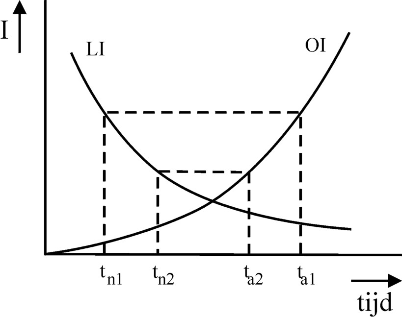
Figure 2: LI and LO and the optimal wage-workingtime relation
The λ is a yet undetermined quantity, and is called the Lagrangians multiplicator. The optimization for respectively ta and tn requires that the partial derivatives of the Lagrangian equal zero. That results in two relations, namely ∂O/∂ta = 1/λ and ∂L/∂tn = -1/λ. After aggregating these two formulas one finds7
(4) ∂L/∂tn = ∂O/∂ta
In analogy with the column about the Robinsonade the formula 4 can be expressed as an identity of intensities of (dis)pleasure8. Then the formula obtains the by now familiar form LI(tn) = OI(ta). This implies that ta is fixed as an automatism at the instant, that a certain tn has been chosen, and vice versa.
Moreover, in the column about the Robinsonade mentioned just now the intensity of pleasure LI turns out to be a falling function (effect of saturation), while the intensity of displeasure OI is a rising function (increasing aversion). Incidentally that is also apparent from the figure 1. The figure 2 shows in a graphic form the developments of the intensities as a function of the time t, for both intensities LI(t) en OI(t). The figure also illustrates in a graphic way the meaning of formula 4, the condition for the optimal solution. It is clear that in the figure the Robinsonade is present as a special case, with ta = tn. The curves intersect each other in the optimum. In all other cases, with ta≠tn, the optimal pair (ta, tn) is not found as the intersection of LI and LO, but as the intersection of the two curves with a horizontal line.
For the sake of convenience in the figure 2 it is indicated for two values of tn (numbered 1 and 2) what the corresponding values of ta will be. The result is somewhat surprising: when tn decreases, then ta increases. A smaller tn implies that the worker is engaged with less time for himself, and consequently his wage decreases. In other words, he obtains less pleasure from his wage. At the same time the increase of ta implies, that his working-day lengthens9. Thus De Wolff finds the following connection: a decreasing wage is accompanied by a lenghtening working-time, and conversely. The lenghtening of the working-day benefices the producer. Note that according to the formula 1 a decrease of tn in combination with an increase of ta implies a rise of the degree of exploitation u.
De Wolff defines the degree of employment z as the fraction of the workers, that is employed. So the possible values of z vary between 0 and 1. In the model of De Wolff the degree of employment is a function of the wage level w. According as the wage decreases, more and more workers will experience insufficient pleasure from the income. An increasing number of them will prefer to stay at home. Evidently that reduces the degree of employment. In a mathematical notation this is z=z(w) and ∂z/∂w > 0. For the present purposes the inverse relation is more practical, that is to say, w=w(z). De Wolff calls w(z) the wage function. Of course the wage sum L(z) rises with an increasing degree of employment z, and also with the wage level w(z). One finds
(5) L(z) / L(1) = z × w(z) / w(1)
In the formula 5 L(1) and w(1) represent the values of these quantities for z=1.
The purpose of this column is to calculate the size of the national product Q. Naturally, the size of that product depends on the degree of employment. Besides Q will depend on the length of the working-day ta. Now in the preceding paragraph it has been shown, that ta is a function of tn, and thus of the wage level w=w(z). The logical conclusion is that ta itself is a function of the degree of employment. The working-day would lengthen for a falling wage. In the mathematical notation this is ta = ta(z), with ∂ta/∂w < 0 and ∂ta/∂z < 0. De Wolff calls ta(z) the function of labour time. Thus the following relation is found for the size of the national product
(6) Q(z) / Q(1) = z × ta(z) / ta(1)
In the formula 6 Q(1) and ta(1) represent the values of these quantities for z=1.
The producers-capitalists strive for a maximal total profit P. Thus the optimal size Qopt of the national product is the one, that has ∂P/∂z = 0. The formula 1 shows, that this condition is identical to
(7) ∂Q/∂z = ∂L/∂z.
This identity can be rewritten further by inserting the formulas 5 and 6. Here it is practical to use also the formula 1, namely Q(1) = L(1) × U(1). Thus one finds
(8) U(1) × ∂(z × ta(z) / ta(1)) / ∂z = ∂(z × w(z) / w(1)) / ∂z
According to De Wolff this is the formula, that determines the optimal degree of employment zopt for the producers in the economic system. All other quantities can be found simply by inserting this zopt in the corresponding functions.
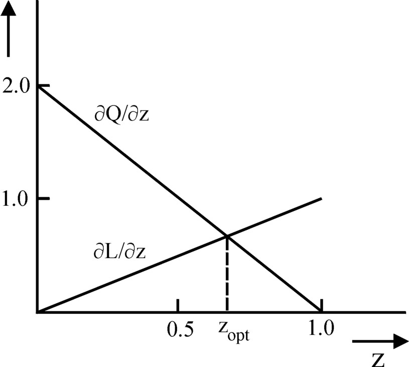
As an illustration De Wolff ends his theory with an example. He takes w(z) = z × w(1) as the wage function,and ta(z) = (2 − z) × ta(1) as the function of labour time. The degree of exploitation is set at u(1)=1, which directly leads to U(1)=2. These functions are all inserted into the formula 8. After some calculations the result zopt = 2/3 is found. Apparently an employment of 67% guarantees the optimal profit for the capitalists. Then the wage has fallen to 2/3 × w(1), while the working-day has risen to 4/3 × ta(1). Now according to the formula 6 the national product equals 8/9 × Q(1), while according to the formula 5 the wage sum equals 4/9 × L(1), or 2/9 × Q(1). The optimal profit is the difference between Q and L, which amounts to 6/9 × Q(1). Finally the degree of exploitation u has become 3 in the optimum. This u is larger than u(1), because the wage has fallen and the working-day has lengthened. Here the cause of the increased exploitation is empathically not the technological progress.
For the sake of completeness the figure 3 also shows ∂Q/∂z and ∂L/∂z as a function of the degree of employment. Here the values of Q(1) and w(1) are put equal to 1, following De Wolff. This only scales and simplifies the vertical axis. It can be checked by means of this figure, that in the optimal point of the formula 7 indeed zopt = 2/3 is valid.
Thanks to the model just described De Wolff has reached his goal. He has succeeded in showing that in capitalism the optimal economic system still has a structural unemployment. However his sense of honour incites him to also study the effect of the technological progress on the system. In the introduction it has been shown how the technological progress amounts to an increasing degree of exploitation. The wage goods keep getting cheaper. Now De Wolff investigates the effect of an increasing exploitation on the optimal degree of employment zopt.
The model calculation allows to rapidly obtain a qualitative impression of the effect. There U(1) is the measure for the technological progress. In the calculation it is found that (see the formula 5)
(9) ∂L(z)/∂z = z × (Q(1) / w(1)) × (2 / U(1))
The formula 9 shows that the slope of ∂L/∂z is apparently inversely proportional to U(1). In the figure 3 the inverse proportionality implies that the slope of the line ∂L/∂z decreases according as U(1) increases. Then, since U(1) does not influence the line ∂Q/∂z, the intersection of the two lines will shift to the right. In other words, in this calculation the increase of U(1) resulting from the technological progress leads to a rising zopt. Thus De Wolff reaches the surprising conclusion, that thanks to the technological progress the degree of employment will improve. This is truly a promising result!
it is probably useful to make the remark, that U(1) does not depend on z, but it does vary with zopt. Both U(1) and zopt are quantities, that in the short run, in a given social episode, characterize the state of the technology. However, in the long run both are variables, and mutually dependent.
De Wolff is not content with the qualitative explanation of the relation between u(1) and zopt, and he searches for a formal derivation. This analysis is not particularly fascinating, but your columnist does present her, because she illustrates the mathematical skills of De Wolff so well. His analysis starts with the observation, that a function χ(z) can be defined by L(z) = χ(z) / U(1) (compare this with the formula 9). Then the optimization of the profit P(z), as it is expressed by the formula 7, takes on the form Q' = χ' / U(1). Here the accent is again the short notation for the derivative to z. Thus a new expression is found for U(1), namely χ'/Q'. This expression is only valid for z=zopt, so that apparently one has U(1) = U(1, zopt). De Wolff wants to know how U(1, zopt) varies with zopt, and therefore studies the derivative dU(1, zopt)/dzopt. A repeated differentiation yields U' = (χ'' × Q' − χ' × Q'') / (Q')2. Next De Wolff notices, that the optimization of the profit P(z) leads to an additional requirement, namely ∂2P / ∂z2 < 0, or ∂2Q / ∂z2 < ∂2L / ∂z2, or Q'' < L'', or Q'' < χ'' / U(1). The reader should notice that here the derivatives are with respect to z, and not to zopt, so that U(1) is still a constant here. De Wolff substitutes the additional requirement in the formula of U', resulting in U' > (U × Q'' × Q' − χ' × Q'') / (Q')2 = (Q'' × (U × Q' − χ') / (Q')2. Finally it follows immediately from the condition for optimization Q' = χ' / U(1), that the right-hand side equals zero. Thus De Wolff has proven in a formal and analytical way, that dU/dzopt > 0. The optimal degree of employment increases with the technological progress, which had to be proven.