
Figure 1: Tile Sint Eloy (1967)
In the book Economic policy: principles and design1 the well-known economist Jan Tinbergen shows that the state can develop a policy for controlling the economy. The policy consists of a set of goals, and the corresponding instruments. The present column describes two models with variable prices and foreign trade, which allow to analyze the policy. The price elasticities are also taken into account. Besides, the first model contains a system of taxes. The models are copied from the mentioned book.
In a previous column several models of Tinbergen have been described, which extend the Harrod-Domar model with price-effects. Tinbergen presents the models for the first time in his book Mathematical models of economic growth2. The present column extends the models from the preceding column with new elements, namely the distribution of incomes, the levying of taxes, and the labour productivity. It is true that this does not yield fundamentally new insights, but it does show the versatility of the method. For the sake of simplicity the productive structure is not included in the models. This implies, that the formation of the stock of capital goods is not addressed. In all cases the system is open, with international trade.
The starting point of any one-sector model of an open economy is the formula3
(1) Y = C + I + EX − IM
In the formula 1 Y is the national income, C is the supply of consumer goods, I the supply of investment goods, EX is the export, and IM is the import. According to Tinbergen the model belongs to the micro-economy, because a distinction is made between the nature of the goods. Your columnist prefers to call it a macro-economic model, because the productive sphere is hardly addressed.
The variables in the formula 1 represent money sums. They are related to the corresponding physical variables c, i and ex by means of the general domestic price level p 4. Notably one has C = p×c, I = p×i, and EX = p × ex. In other words, the consumer goods and the capital goods have a single price level, and the export prices are identical as well. Thus the total material national product is q = c + i + ex. Tinbergen assumes, that the import satisfies IM = pIM × im = pIM × ι×q. Here pIM is the price level of the import goods, and ι=im/q is the import rate. Apparently a larger national product increases the import. Note, that here the import rate is related separately to the phyical variables. The price ratio p/pIM (the terms of trade) has at most an indirect influence. The difference D = IM − EX is called the deficit on the balance of payments.
The domestic price level gets in the present model a form, that has already been discussed in the previous columns about the theme, namely
(2) p = po × qμq × pLμL × pIMμIM
The right-hand side of the formula 2 is commonly called a Cobb-Douglas function. The formula 2 distinguishes between three causes of price inflation. First, an increase of q will cause rising costs. This is actually simply the inflation, resulting from demand pull and cost push. In addition the rising costs due to the increasing wage level pL is taken into account, also called wage inflation. And finally the costs can rise, when the import becomes more expensive, so that the inflation is imported. The constant coefficients μq, μL and μIM are the corresponding price elasticities5. Although the price elasticity μex of the export does not enter in the formula 2, she does evidently matter for the size of q.
The model distributes the consumption over three social groups, namely the public sector, the wage-dependent workers, and the capitalists with their unearned incomes. Such a C, which takes into account the public sector, is called the consumption against factor costs6. The public sectors obtains its income among others by levying the sales tax τi (i from indirect). This tax is passed on to the consumers, so that the price level on the market is p+τi7. Incidentally, this tax is not paid for investment goods or export goods, as is well known. Therefore the consumption against market prices has a value Γ = (1 + τi/p) × C. If desired the price level on the consumer market can be defined as p' = p + τi, so that the consumption against market prices can be rewritten as
(3) Γ = p' × c
Now the income distribution can be divided further. The total gross wage sum is W = pL × ν×L, where ν represents the employment, as a fraction of the total professional population L. The symbol W represents the word wage. The workers are not completely free in spending their income, because they must remit an income tax tau;L on pL to the state. For the sake of convenience it is assumed here, that the remittance is returned completely to them in the form of various public services. Besides, the state consumes a given sum Co. The total unearned income is P = Y − W (P from the word profit). Tinbergen puts the tax burden on P equal to θP, in this case indeed as a fraction of P. The capitalists do not receive public services in return. In other words, the capitalists keep a nett income P = Y − W 8.
Next the total expenditure or consumption function can be derived. It is assumed, that the state and the workers spend their whole income on consumer goods. However, the capitalists will consume merely a part of their nett income, namely γ × (1 − θP) × P. In this expression γ is the so-called rate of consumption of the capitalists. The capitalists invest subsequently the remainder of their income. So in this model the capitalists are the only ones, who truly invest - unless one would allow for an investment component in Co. Thus the toal social consumption function and the investment function obtain the forms
(4a) Γ = Co + W + γ × (1 − θP) × P
(4b) I = (1 − γ) × (1 − θP) × P
If desired the labour productivity can be included in the model, in the form ap = ν×L/q. Furthermore it must be noted, that the price elasticity μx of some variable x is defined as -∂x/∂p / (x/p). Here the minus sign is added in order to yield a positive elasticity, at least as long as it is assumed that a rising price reduces the quantity of x. Thus the price elasticity μex of the export can be used to derive ex = exo × p-μex. Here exo is a proportionality constant. This completes the mathematics of the model. It is interesting, that the formulas in this model can be reordered in such a manner, that the calculation of all variables is fairly simple.
The mentioned reordering proceeds as follows. The policy maker chooses the variables, that will serve as policy goals. According as more goals are selected, also more policy instruments will have to be employed. The loyal reader recognizes this rule of thumb from the previous column about models with a money market. But there the number of policy goals is low, namely merely two. Here that number will be increased, to four goals. For instance, start with the employment ν as the first variable and policy goal:
(5a) q = ν × L / ap
(5b) im = ι × q
(5c) IM = pIM × im

Apparently one has q = q(ν), im = im(ν) (because im = im(q)), and IM = IM(ν). All these variables follow directly from ν, because Tinbergen assumes that L, ap, ι and pIM are constants. When the value of the goal ν has been chosen, then all variables from the group [q, im, IM] are fixed. However, Tinbergen believes that they are not convenient for using as an instrument. Therefore, first a second variable and policy goal is added, besides ν, namely the deficit D of the balance of payments. For, that must be controlled, because a durable deficit can not be maintained economically. It follows that:
(5d) EX = IM − D
(5e) p = EX / ex
(5f) ex = exo × p-μex
Apparently one has EX = EX(ν, D). The formulas 5e and 5f are mutually coupled. The formula 5f expresses, that one has ex = ex(p). Therefore the formula 5e equals p = p(EX, ex(p)), and from this it follows that p = p(EX) = p(ν, D). Then one also has ex = ex(ν, D). The chain continues:
(5g) pL = pL(p, q) (due to the formula 2)
(5h) Y = p × (q − ex) − D
(5i) W = pL × ν × L
(5j) P = Y − W
Thus one has pL = pL(ν, D), Y = W(ν, D), W = W(ν, D) and P = P(ν, D). Tinbergen states that the group [EX, p, ex, pL, Y, W, P] contains a valuable instrument, namely the wage level pL. But the other variables in the group are ill suited for the role of instrument. As the third variable and policy goal the physical investment volume i is chosen, because it affects the economic growth. Then the calculation can proceed:
(5j) I = p × i
(5k) c = q − i − ex
(5l) C = p × c
(5m) θP = 1 − I / ((1 − γ) × P)
Apparently this group of variables exhibits the behaviour I = I(ν, D, i), c = c(ν, D, i), C = C(ν, D, i), and θP = θP(ν, D, i). The group [I, c, C, θP] clearly contains an effective instrument, namely the tax-load θP on the unearned incomes. For, it is directly imposed by the state. The fourth and finally added variable and policy goal is the domestic price level p'. It is suited well for the stabilization of the prices, so that the inflation is curbed. The definition of p' immediately yields
(5n) τi = p' − p
Next one also has
(5o) Γ = p' × c
(5p) Co = Γ − W − γ × (1 − θP) × P
That is to say, one has τi = τi(ν, D, p'), Γ = Γ(ν, D, i, p'), and Co = Co(ν, D, i, p'). Here the choice of an instrument is also obvious, namely the sales tax τi. Besides, the state expenditures Co are a convenient instrument, because the state can control them. Thus Tinbergen shows, that the policy goals of employment, an equilibrated balance of payments, the physical investment volume, and the price level for consumer goods can be realized by chosing the right values for the wage level, the state expenditures, and two types of taxes (namely, direct and indirect ones).
Tinbergen gives on p.122 of his book Economic policy: principles and design a scheme with arrows, which is reproduced in the figure 5a-p as a causal chain. He supplements it with a so-called order of Simon. Although that scheme is definitely instructive, your columnist omits its, because it is somewhat difficult to draw. Both the scheme and the order of Simon illustrate again the causal relations in the chain. Starting from q in the formula 5a one ends at Co in the formula 5p. The policy goals form the starting points of the calculation, as it were, and the policy instruments form the endpoints.
The order of Simon refers to the critical path length in the scheme. Thus the longest path has nine links: q → im → IM → EX → p → pL → W → P → θP → Co. In this path q is of the zeroth order, and Co is of the nineth order. The construction of the path starts at its end. Thus some paths do not have links of the lowest order (0, 1, 2 etcetera). Note, that the model uses a total of 17 variables, namely q, im, IM, EX, p, ex, pL, Y, W, P, I, c, C, θP, τi, Γ, and Co.
Tinbergen shows, that the set 5a-p can be simplified by expanding all variables X in a truncated series around an initial value X(0) at t=0. The assumption is, that these initial values X(0) are all given. A period Δt later one will have X(Δt) = X(0) + ΔX. It turns out, that all formulas 5a-p take on a linear form, when they are expressed in the change ΔX instead of in X itself. Here it is assumed, that ΔX is small in comparison with X, and therefore all quadratic terms ΔX1 × ΔX2 may be neglected (small squared is nothing). It the same way ΔX / X(Δt) is replaced by ΔX / X(0). Etcetera. In this approach one does not calculate X(Δt), but ΔX. The advantage of linear relations is obviously, that they are convenient in calculations. Moreover, the policy makers are often mainly interested in the changes.
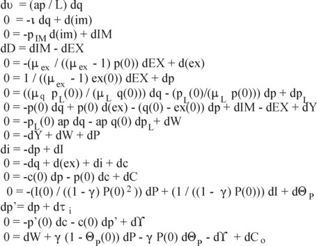
Instead of the mentioned 17 variables, there are now 17 changes, say ΔXk, with k = 1, ..., 17. This can be interpreted as a vector ΔX. Tinbergen shows, that the vector satisfies the vector equation B = A · ΔX. In this equation B is a vector, that contains the policy goals, and furthermore merely zeros. The symbol A represents a 17×17 matrix, which almost has a triangular shape (merely zeros above the diagonal). In the figure 1 the components and elements of B, A and ΔX are shown. Now ΔX can be calculated from A-1 · B, where A-1 is the inverse matrix of A. The disadvantage of this linearization method, which incidentally Tinbergen often employs in his book, is that the relations become rather sloppy and they lose their self-evident logic.
This paragraph discusses a model, where the labour productivity ap is variable. Since several sectors n are present (n = 1, ..., N), the system is described at the micro-economic level9. The model is especially useful in illustrating the consequences of an increasing ap on the economy. The obvious advantage is, that the goods become cheaper, so that the spending power of the income increases. However, a surprising disadvantage is that the domestic price level p falls, because this worsens the terms of trade p / pIM 10.
The national income is
(6) Y = Σn=1N (Xn + EXn − IMn)
In the formula 6 Xn is the domestic consumption of the product n. No distinction is made between the consumption and the investments. Tinbergen assumes that the expenditure function is given by Xn = ξn × Y, where ξn is the expenditure ratio for the product n. The other terms in the formula 6 represent the export and the import.
All variables can obviously be transformed into the corresponding physical variables. Thus the physical consumption equals xn = Xn / pn, where pn is the market price for the product n. In the same manner the physical export equals exn = EXn / pn. The transformation of the import requires the import price pIM, so that then one has imn = IMn / pIM,n. Define also qn = xn + exn, then one has imn = ιn × qn, with ιn representing the import ratio of the product n. The foreign demand for the product n varies obviously with the product price, and this market behaviour is described by the price elasticity μn of the export. The deficit on the balance of payments is D = Σn=1N (IMn − EXn).
The labour-productivity apn is defined as qn / Ln, where Ln is the number of workers in the sector n. Suppose that the productivity apn rises, whereas the production costs do not change. Then xn and exn increase, but Xn and EXn do not. In other words, pn changes in an inverse proportion with apn. In mathematical terms this is pn = po,n / apn, where po,n is a suitably chosen constant. This remark completes the model. The remainder is a simple elaboration of the preceding formulas.
Some simple reformulations lead to11
(7) IMn = ιn × (pIM,n / pn) × (Xn + EXn)
Use the formula 7 for eliminating IMn from the formula 6. Then one has
(8) Y = Σn=1N (1 − ιn × (pIM,n / pn)) × (Xn + EXn)

The formula 5f is also here useful for the calculation of exn, and thus also of EXn. Insertion of this EXn and of Xn = ξn×Y leads, after some reformulation, to
(9) Y = [Σn=1N (1 − ιn × (pIM,n / pn)) × exo,n × pn1-μn] / [1 − Σn=1N (1 − ιn × (pIM,n / pn)) × ξn]
Designate the term in the numerator with the symbol Λ. In other words, let
(10) Λ = Σn=1N (1 − ιn × (pIM,n / pn)) × exo,n × pn1-μn
Then one has according to the formula 6
(11) D = Y × (-1 + Σn=1N ξn) = Λ × [-1 + Σn=1N ξn] / [1 − Σn=1N (1 − ιn × (pIM,n / pn)) × ξn]
Tinbergen applies the model to the situation, where the policy maker chooses the employment and the equilibrated balance of payments as his policy goals. He wants to use the labour productivity in two sectors as his instruments, for instance n=1 and n=2. Then the argument can henceforth be restricted to these two sectors. Your columnist is so bold to deviate from the remainder of the argument in Economic policy: principles and design. Instead the argument is as follows: suppose that Σn=1N ξn > 1. Then according to the first step of the formula 11 the variable D must be positive. There is a deficit. Suppose for the sake of convenience, that Λ is also positive. That is for instance the case, when one has ιn × (pIM,n / pn) < 1 for all n. Then curbing the deficit implies, that Λ must be reduced.
What is now the effect of an increase of the productivity apn on Λ and D? It will push down the product price pn. Therefore in the formula 10 the factor (1 − ιn × (pIM,n / pn)) will get smaller. But the effect of the lower pn on pn1-μn is less clear. For the case of a price elasticity μn < 1 this term will also decrease. However, as soon as the elasticity satisfies μn > 1, then this term will increase. This may well have the effect, that due to the rising productivity Λ will become larger, and thus also the deficit D. In other words, in spite of the increasing efficiency of the domestic production, the trade with foreign states is undermined!
Next consider the second policy goal, that of the employment L. It is12
(12) L = Σn=1N qn × pn / pon
In the preceding calculations it has already been shown, that one has qn = Y × ξn / pn + exon × pn1-μn. Apparently then one has
(13) L = Y × Σn=1N (ξn / pon) + Σn=1N (exon / pon) × pn1-μn
What is the effect of the increase of the productivity on L? On the one hand, the reduction of Λ, which is needed in order to curb D, will also push down Y, according to the formulas 9 and 10. The first term on the right-hand side of the formula 13 decreases. For the second term on the right-hand side there are two possibilities. When μn < 1 holds, then the increase of the productivity will push down also this term. Then the employment clearly diminishes. However, when μn > 1 holds, then the second term will rise. The interaction of the two terms on the right-hand side in the formula 13 will determine how the employment will develop.
In conclusion: it would seem, that the increase of the productivity leads to a larger product demand from abroad, and to more export. However, the falling product price undermines the terms of trade, so that the deficit on the balance of payments increases, in spite of the reviving physical (material) export. The employment can also decrease. The surprising results of this model are an incitation to always maintain a critical view on the causal relations in the system during a policy analysis. And although Tinbergen does not mention it, the abstractions in the model itself must be scrutinized as a possible source of unrealistic results.