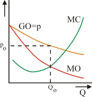
Figure 1: p, MO and MC versus Q
It is sometimes argued that unemployment can be reduced by a targeted wage policy. This column analyzes the relation between the wage level and newly created of jobs. First, the employment in a single enterprise is studied, with the neoclassical paradigm. The scale- and substitution-effects due to a changing wage level are analyzed, in the short and long run. Next the problem is modeled by means of the neoricardian theory. Finally a macro-economic model of Jan Tinbergen is presented.
The present high unemployment in Europe and especially in the Netherlands incites to search for policy solutions. In the traditional neoclassical paradigm a decrease of the wage level would lead to extra employment. The political discourse in the Netherlands accepts this idea without criticism, both at the left and right side, and within circles of both entrepreneurs and trade unions1. That is strange, because on this portal references are regularly made to the neoricardian paradigm, which does not predict a simple ("logical") relation between the wage level and the employment. In the present column the deficiencies and misconceptions in the neoclassical paradigm are again summarized. Besides, a model of Tinbergen is presented, that shows the possible absence of the "logical" relation as a result of differences in the behaviour of spending.
First a study is made of the manner, in which the wage level affects the employment in a single enterprise. Here notably the chapters 2-4 in the book Modern labor economics are consulted2. The starting point of the argument is the neoclassical production theory. In the neoclassical paradigm the enterprise is simply the place, where the production factors such as labour L and the capital goods K (from the German wordt Kapital) are combined in order to generate a certain end product. Suppose that the production quantity is Q units, then the enterprise equals the production function Q = f(L, K). The function f is the mathematical representation of the technological production process, which is used by the enterprise.
In the neoclassical paradigm labour and capital can mutually be substituted (exchanged), so that a certain quantity Q0 of the product can be produced with all kinds of combinations of L and K. In other words, the enterprise can choose from an infinite number of techniques. The collection of points (L, K), which belongs to the quantity Q0, is called an isoquant. It is commonly assumed, that the isoquants have a convex shape in the (L, K) plane.
According to the neoclassical paradigm the behaviour of the enterprises is determined by the desire to maximize the profit π. The price of a unit of the product is represented by p. Let W be the wage level (rate), and R the price (rent) of a unit of capital. Then the profit is
(1) π = p × Q − (W × L + R × K)
In the formula 1 p×Q is the total revenue TO of the production, which also implies that p equals the average revenue GO per unit of product. The profit is computed by subtracting the costs from TO. It is clear, that the costs are typical for each enterprise, and they are represented by the cost function C(Q). The profit is maximal in the point Q*, where one has ∂π/∂Q = 0. Thanks to this condition the formula 1 can be rewritten as
(2) p + Q* × ∂p/∂Q = W × ∂L/∂Q + R × ∂K/∂Q
In the formula 2 the values of the derivatives of the functions must be computed for the optimal quantity Q*. It is assumed that W and R do not depend on the quantity Q. The left-hand side of the formula 2 is called the marginal revenue, in short MO, so that one has MO = ∂TO/∂Q. For, the differentiation with respect to Q is a way to calculate the extra revenue, which is created due to the production of an extra product unit. Stated differently, the variable MO approximately equals the quotient ΔTO/ΔQ, where ΔQ is a small quantity and ΔTO is the corresponding revenue. The right-hand side of the formula 2 is called the marginal costs, abbreviated as MC. Then one has MC = ∂C/∂Q.
In short, the maximization of the profit leads to the identity MO = MC. Note that in the formula 2 the derivative ∂p/∂Q must be negative. For, the neoclassical paradigm assumes equilibrated markets, which are cleared completely. An increase of the sales is only possible by a reduction of the product price. Due to the negative derivative the marginal revenue MO is smaller than the price p (which equals GO). This phenomenon is illustrated in a graphical manner in the figure 1. The curve p(Q) is simply the market demand for the product. On the one hand the last sold product unit adds a sum p to the revenue. But on the other hand each extra sold unit pushes the price downward, so that the preceding units will yield less. Therefore one has MO<p.
It was just mentioned that the right-hand side of the formula 2 represents the marginal production costs due to the factors labour and capital. The figure 1 shows that the enterprise will expand its sales as long as MC is less than MO. For, on all those product units a profit will be made. Besides, the figure 1 shows that MC(Q) is rising, at least for the larger quantities. The rising costs impose an upper limit for the expansion of the production size to the enterprise. This aspect is the hallmark of cost functions, and deserves a closer inspection. The formula 1 shows, that in the now following argument the derivatives ∂L/∂Q and ∂K/∂Q will play an essential role.
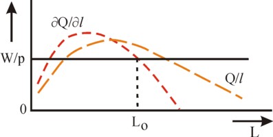
Define the marginal product MPL of labour as ∂Q/∂L, where evidently the quantity of capital is kept fixed. Define also the marginal product MPK of capital as ∂Q/∂K, for a fixed value of L. Note that MPL and MPK are in fact marginal productivities of a unit of the concerned factor. As an illustration the figure 2 gives a graphical sketch for the factor labour. It turns out that the curve peaks at an L value, that fits technically best with the given quantity K. For, K represents simply the machines and equipment,that require operation with a fixed number of workers, because of the technical design. The enterprise will hire workers at least until the peak is reached, because before the peak each extra added worker is more productive than the previous one.
That changes after the passage of the peak due to additional hiring of labour, because then the marginal productivity of labour starts to fall. One has too much labour in comparison with the available capital, as it were. In that domain the derivative ∂Q/∂L is a falling function (and naturally a similar argument can be held for ∂Q/∂K). Furthermore one has ∂L/∂Q = 1 / (∂Q/∂L) and ∂K/∂Q = 1 / (∂Q/∂K), at least as long as Q(L) and Q(K) exhibit a monotonous increase in the pertinent domain3. In other words, apparently the derivatives ∂L/∂Q and ∂K/∂Q must rise for an increasing Q. This is precisely the behaviour of MC, that is visible in the figure 1, and which yet had to be explained.
What are the consequences of the law of the decreasing marginal utility of labour and capital? What does the law imply for the employment in the enterprise?4 In answering this question commonly a distinction is made between the short and the long run. In the short run the enterprise can not expand her capital, because the capital goods must first be ordered, produced and delivered. Therefore in the short run only the manpower L can be varied. Consider again the figure 2. Beyond the peak for each additional worker his produced value must be computed and compared with his costs. The production of the worker is simply the marginal product MPL, and its value is WMPL = ∂(TO)/∂L = (∂(TO)/∂Q) × (∂Q/∂L) = MO × MPL.
Each unit of labour costs W, so that the hiring of workers must stop at the value L*, where one has WMPL = W. In short, the maximization of the profit dictates the following condition for the manpower:
(3) MO(Q*) × MPL(L*) = W
The formula 3 is a special case of the formula 1, because K is constant in the present situation of the short run. In practice the formula 3 is merely applicable for two special types of markets, namely the private monopoly and the perfect competition5. Since the private monopoly is considered to be socially undesirable, she is prohibited by all kinds of market laws. Therefore in this argument exclusively the perfect competition is considered.
The perfect competition is a market form, where each separate enterprise contributes little to the total product. Therefore the separate enterprise can not manipulate the product price. For, since the production of each enterprise is relatively small, the sales of the enterprise do not change the price. The product price is determined exclusively by the supply of all enterprises together. The separate enterprise is a price taker, as it were.
Apparently in the formula 2 the identity ∂p/∂Q = 0 can be inserted. So in this situation one does have for the optimum Q* that MO=p. The formula 3 changes into
(4) MPL(L*) = W / p
The term W/p is called the real wage rate of the enterprise, because he expresses the wage rate in terms of the number of equivalent product units. Apparently the marginal product exactly equals the real wage for the optimal manpower L*.
After all these preliminary considerations now the effect on the employment in the enterprise can be studied, for the case of a falling wage rate W. The reverse case of a rising wage leads to exactly the reverse effects, and is therefore not further discussed. When W falls, and p remains constant, then MPL can also fall. The figure 2 shows, that in this situation the employment L* will rise. This is the relation, which is presented so often in popular textbooks. But this argument has several deficiencies. It is only true, as long as the enterprise can agree in exclusive negotiate with its workers to lower the wage rate, whereas her competitors continue to pay the old higher wage rate. And that is not the usual situation.
The wage rate is commonly determined for the whole branch by collective bargaining between the entrepreneurs and the trade unions. And even when the union is missing, then the enterprise can not simply pay a smaller wage than her competitors, because she would thus lose her personnel. In short, when the wage is reduced, then this happens in the whole branch. And this must affect the product price. For, according to the formula 1 the lower wage implies a reduction of the costs. Due to the market form of perfect competition all enterprises must pass on this savings on costs in the product price, paid by the consumers.
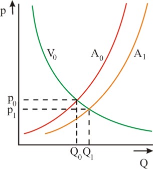
In other words, the decrease of W forces all enterprices to reduce their prices. The figure 3 shows the effect on the market of the product. The price reduction has shifted the supply curve A0 of the whole branch to the right and downward, to the position of A1. Since the demand curve of the consumers does not change, the new supply will lead to an incrase of the total demand for the product. A new market equilibrium is reached, where the totally sold quantity QT,1 of the product is larger than QT,0. It is obvious that this development must be accompanied by a rise of the total employment LT in the branch. This effect of the wage reduction is called a scale effect. This concludes the explanation in Modern labor economics. When the total employment in the branch rises, then this is evidently also the case for the separate enterprise6.
Yet the alert reader will probably agree with your columnist, that this reasoning in Modern labor economics is not complete. First there is the problem, that the product will be used in some other branches as a raw material, a semi-manufactured article, or a capital good. Therefore the lower price results in reduced costs in those other branches. The enterprises in the concerned other branches are evidently also forced to reduce their prices. It is unclear which of those branches will have an increased sales due to those price reductions, and thus have more employment. It is even conceivable, that some branches have a reduced sales, inspite of its reduced production price. The authors of Modern labor economics could at best object, that this is an effect in the long run.
But there is another problem with the reasoning in Modern labor economics. When in a branch the wage rate W is lowered, then its production workers lose some of their spending power. On the other hand perhaps additional workers are hired due to the reduced price. But nevertheless the total spending power W×LT of all workers in the branch could be lower after the wage reduction than before. It is possible that the effect of spending power is neglected in Modern labor economics, because it concerns merely one branch of the whole economy. But as soon as the wage reduction is realized in the whole economy, in all branches, then the effect does require to be taken into account.
The conclusion is that the authors of Modern labor economics restrict themselves to the micro level and do not take into account the macro-economic effects. And that is a mistake. For, when the spending power of the workers in a branch decreases, then they will buy less products. That negatively affects the market demand in all branches. On the other hand, it has just been stated, that in various branches the product prices will fall, so that the spending power of the figure 3 will shift. That effect is reinforced, when the wage reduction is realized in the economy as a whole, in all branches. Your columnist does not see, how in that situation, with the combination of price reductions and lower spending powers, still something meaningful can be concluded about the total aggregate employment in the economy.
After the analysis of the employment effects in the short run, now the effects in the long run must be studied. The long run refers to such a long time, that the enterprise can also change her stock of capital goods K. That is to say, the enterprise can select a completely different production technique. The formula 1 shows, that after a wage reduction the enterprise will search for an alternative technique, that produces as much product Q0 with less capital and (evidently) more labour. In fact the enterprise tries to find the optimal combination (L, K) on the isoquant. In other words, the enterprise wants to replace units of capital by units of labour. Capital is substituted by labour.
Also here merely the case of complete competition is discussed. Suppose that the price p is given, than it is irrelevant, whether the isoquant displays a certain quantity Q0 of the product, or the corresponding total sales TO0. In the column about the production factors it has been shown, that in such a situation the maximization of the profit leads to the requirement
(5) MPL / W = MPK / R
The formula 5 is actually a generalization of the formula 4. The movement across the isoquant is done in steps, as it were, where infinitesimally small steps dL (at a constant K) are alternated with dK (at constant L). The formula 5 guarantees, that for each expended monetary unit for the production factors always the same quantity of product is generated. Besides, the formula 5 illustrates clearly, how the substitution evolves, when the wages fall. For, the decrease of W affects the identity in the formula 5. The identity can be restored by lowering MPL and raising MPK. The figure 2 (and the equivalent for K) shows that this requires an increase of L, and a decrease of K. Apparently in the long run the employment can rise due to its substitution for capital. This is called the substitution effect7.
However, Modern labor economics points out, that the wage reduction does not just cause substitution. On the contrary, primarily she causes a scale effect. Besides the substitution, which constists of the movement across the isoquant, the larger scale of the production causes a movement towards higher isoquants. Thus it is even conceivable, that inspite of the replacement of capital by labour the enterprise will in the end use more capital than before the wage reduction. In that situation L and K are called gross complements, because in the end they both have increased. It is true that this phenomenon is not relevant for the question of employment, but it does illustrate the possible surprises in the development.
In the case of the long run effects Modern labor economics does not address the influence of the price reductions on the product prices in other branches. Neither is the development of the spending power addressed. And that is curious. Namely, the costs of the enterprise are the incomes of others, namely the workers and the owners of capital. An enterprise, which minimizes her costs, also minimizes the spending power. When due to the substitution effect capital is scrapped, then the rentiers lose a part of their income. Similar to the short run case it remains unclear how the product price effects and the spending power effects affect the employment.
The neoricardian theory of Piero Sraffa is a popular theme on this portal, most recently in the column about the reswitching of production techniques. She is strikingly different from the neoclassical paradigm. Some differences are of minor importance. For instance, in the neoricardian society the enterprises aim to maximize the capital efficiency, and not merely the profit. The theory uses merely a uniform wage rate W, and can not differentiate her with respect to the separate branches. And the neoricardian theory is not very informative with regard to demand curves of the various product markets and the like. But she does show in an excellent manner the influence of the wage rate W on all product prices, and on the choice of a certain production technique.
In particular the neoricardian theory proves, that a falling wage rate W does not necessarily lead to the just described substitution effect. On the contrary, a falling W causes a rather inscrutable succession of production techniques, where even a previously abandoned technique can later be preferred. This phenomenon is called reswitching. The development looks so chaoticly, because she is dictated at the macro level, and not at the level of the enterprise or branch. Thus it is conceivable, that inspite of a falling W some branches will prefer a technique with less labour. These phenomena are unfortunately ignored in Modern labor economics.
Finally a macro-economic model is discussed, which the well-known Dutch economist Jan Tinbergen has proposed in his book Economic policy: principles and design8. This model shows that a fall of the general wage rate affects the general employment. A surprising aspect of the model is, that this influence is partly determined by the consumption behaviour of the population. Thus under certain conditions a falling wage rate can still hurt the employment, even when phenomena like reswitching are ignored.

The starting point of the model is the national income y. The wage sum in the national income is ω = W×L, where W is the wage rate and L is the employment, as before. The capital owners (the rentiers) receive the remainder ρ = y − ω as their income. The wage earners spend a part ξl×ω + ηl of their income, and the rentiers spend a part ξr×ρ + ηr. Here the loyal reader recognizes a variant of the consumer functions9. In the formulas ξl and ξr are the so-called marginal spending quotes, whereas ηl and ηr represent the autonomous expenditures of the two groups. The aggregated expenditure of the two groups is ξr× y + (ξl − ξr) × ω + ηl + ηr.
In a situation of equilibrium the expenditures will equal the national income y. Besides the expenditures must equal the value of the total product p×Q, where p is the general price level, and Q the demand on the markets. In other words, the total product and the market demand coincide, so that the market is cleared. This leads to the formula10
(6) p × Q = ((ξl − ξr) × ω + ηl + ηr) / (1 − ξl)
The price level p depends on the costs. It is obvious that the wage rate W affects the production costs, and thus p. But also the size Q of the market demand pushes the costs upward, because the marginal product of the production factors is a decreasing function of Q. See the figures 1 and 2. Thus the price level can be written as11
(7) p = p0 × Wμ1 × Qμ2
In the formula 7 μ1 and μ2 will usually be positive. Furthermore, it is assumed, that the employment depends on the demand Q according to the formula
(8) L = L0 × Qλ
Note that in the formula 8 the variable (Q/L) / λ equals the marginal product of labour. Intuitively one would expect λ>0. However, the preceding discussions have shown that at the macro-economic level the various so-called matters of course are lost. In any case it is immediately clear, that the set of formulas 6-8 allows for the mathematical calculation of the employment L as a function of the wage rate W. Define for the sake of convenience ξ = (ξl − ξr) / (1 − ξl). After some elaborate calculations one finds12
(9) ∂W/∂L = (ξ×W − ((1 + μ2) / λ) × p×Q / L) / (μ1 × p×Q/W − ξ×L)
The formula 9 is still not very transparent. Therefore on p.232 of Economic policy: principles and design Tinbergen takes for the sake of convenience as values W=1, p=1, Q=1 and L=½. This means that the wage sum ω is half of all expenditures. In that situation it is realistic to choose μ1=0.4, μ2=0.2, and λ=0.4. Insertion of these values considerably simplifies the formula 9:
(10) ∂W / ∂L = (12 − 2 × ξ) / (ξ − 0.8)
The formula 10 shows that for this situation the derivative will be positive for ξ-values between 0.8 and 6. In that domain a falling wage will apparently cause less employment! Furthermore, note that the marginal expenditure quotes must be less than 1. Therefore the condition ξ>0.8 implies that one must have ξl > ξr. In other words, the workers spend a larger fraction of their income than the rentiers. This is the cause of the surprising causal relation ∂W/∂L > 0.
In the neoclassical logic the reduction of the wage must lead to more employment. Namely, according to the price formula 7 the price level is pushed down by the falling W. According to the expenditure formula 6 a falling price level p results in a rising market demand Q. And according to the formula 8 this increases the employment. However, the term (ξl − ξr) × ω in the expenditure formula 6 interferes with this reasoning, for it will fall due to the decreased wage rate. Therefore the demand Q can not grow, but it must even shrink. The redistribution of income, that is the consequence of the lowered wage, gives an extra spending power to the rentiers, who however do not use it! And although the model of Tinbergen has obvious limitations, it clearly illustrates here that the consequences for the employment of shifts in income are untransparent.