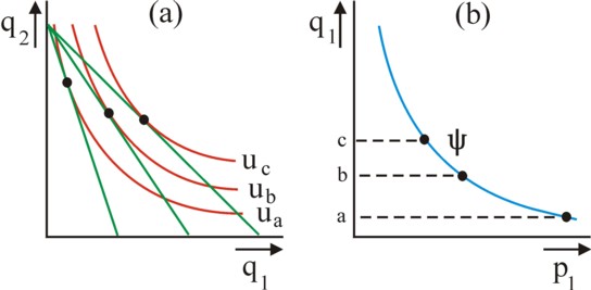
Figure 1: (a) indifference curves and budget lines
(b) normal demandcurve ψ, belonging to figure a
The present column describes several essential concepts and models of welfare economics. First the compensated demand curve, the consumer surplus, the rent of entrepreneurs, and the dead-weight loss are explained. Next, measures of social inequality are discussed. They are convenient in order to include the aversion against inequality in the social welfare function. The economist Binmore shows, that the latter inclusion can also be realized by combining the pure utilitarianism and the maximin principle of Rawls.
The consumer behaviour of the individual k is commonly determined by two factors: his preferences and his income yk. Preferences can be modelled as a utility function uk. The individual makes his choices from the assortment of products, which is available on the markets. Suppose that the market offers N differing consumer goods, with a market price pn for product n. When saving is ignored, then the consumption of k is limited by the so-called budget line
(1) yk = Σn=1N pn × qn
Here qn is the quantity of the product n, which is consumed by the individual k. Actually pn and qn are vectors with N elements each, so that for the sake of convenience the formula 1 can be represented by the inner product(p·q). The vector q transforms the income yk in a basket of commodities. Common sense says, that q depends on p. For, expensive products are less desirable. The function qn,k(p) is called the individual demand curve of the product n, in agreement with the preference of k. The form of the demand curve can be derived analytically. Namely, the individual k naturally tries to optimize the utility of his basket of commodities, within the limits of his income. The optimal composition is given by qk*. Incidentally, for the present discussion it is more clarifying to interpret the utility as the welfare of k. The consequence is, that qk* is determined by the utility function uk(q) of k. For the sake of convenience the index k will be omitted in the notation.
For the sake of clarity the analysis of the demand curve is commonly presented in two dimensions. In this way the problem can be shown as a graph. Thus the figure 1a presents the utility field u(q1, q2) of an economy with two products (N=2). Each red curve is an indifference curve of constant utility, with a rising welfare in the order ua, ub, and uc. Now suppose that the product price p1 of the product 1 is reduced in steps, with p1,a > p1,b > p1,c. The price p2 remains constant. This is actually a deflation, because the spending power per unit of money rises. Since the individual income y has a nominal value, in this situation the individual welfare increases. This phenomenon is shown in the figure 1a. The green lines are the budget lines for the same y, but at three different prices p1. According as p1 falls, the optimum q* shifts: the individual gives up units of product 2 in order to acquire more units of product 1.
The process of optimization can be called a utility maximization problem, or an expenditure-minimization problem1. Apparently two mechanisms are relevant. On the one hand there is substitution of the product 2 in favour of the product 1. The Gazette has paid attention many times to the substitution of production factors, and the same process occurs here for decisions about consumption. On the other hand, the individual can buy more of both products, because his real spending power has increased. Thanks to the extra spending power with a size of q1 × Δp1 the individual welfare obviously increases, from ua to ub and uc. This second phenomenon is called the income effect. Within this frame, a convenient concept is the expenditure function, which is defined as e(p, u) = y(q*). Although y remains constant, both p and u change.
The figure 1a is especially interesting, because for each value of p1 the corresponding optimal q1* can be read. The resulting curve is shown in the figure 1b. This is called the normal demand curve ψ1(p1,y), or also the demand curve of Walras or Marshall2. Note that in graphs the demand curve is often confusingly presented with q* along the horizontal axis and p along the vertical one! This ignores the causality. Since ψn can be determined for all n products, it is actually a vector ψ. The function ψ plays an important role in the study of market processes, However, it is not suited for describing the development of welfare. For, in changes of p1 the individual utility u varies in a complex manner.
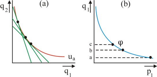
Therefore economists have invented an alternative demand curve, which has little practical relevance, but which is indispensable in welfare theory. Consider for this the figure 2a, which shows the indifference curve ua. It has just become apparent, that the income y in combination with the product price p1,a leads to the optimal consumption qa* on the curve u=ua. This budget line is drawn in the figure 2a. Also all other points on the curve represent an optimum q*, with the same utility ua, but at another price p. As an illustration two are drawn, for p1,b and p1,c, with unchanged p2. The three green lines are again budget lines, where however only qa* still has e(p,u) = y. For, the falling p1 increases the spending power, so that the utility ua only remains constant for a falling income e(p,ua). The points on u=ua define the compensated demand curve q1* = φ1(p,u). This function is also called the demand curve of Hicks3.
The income y no longer appears in φ, because it naturally adapts to p1 and ua. For instance, the income falls between qa* and qb* with e(pa,ua) − e(pb,ua) 4. This is an abstraction, because actually the households and companies always have a budget limitation. The income effect is eliminated artificially from the theory. Therefore the price p can not be attributed here to the market process. In the compensated demand curve the individual does not optimize his basket of commodities, but expresses with pn his personal appreciation for the product n. Then pn is called the marginal evaluation, or the willingness to pay5. A simple use is made of the second law of Gossen, which states that the unit price matches the marginal utility. In formula: ∂u/∂qn = λ×pn, where the so-called marginal utility of the expenditure λ is a constant for all products n.
In other words, the acquisition of the product n is indifferent. The price and the individual (marginal) utility are balanced. An outsider can only measure the compensated demand curve φ by asking the individual about it. The function φ can be constructed from the utility field, with the same method, which has been applied in the figure 1 for the demand function ψ. Then the compensated demand curve in its common form is found. The result is shown in the figure 2b. Note that φ1(p1,ua) falls in a less steep manner than ψ1(p1,y) 6. Now suppose, that the product n is offered for a unit price of πn. Then the individual continues to buy units of the product, as long as πn ≤ pn holds. In other words, he obtains the units qn = φn(πn,u) at a lower price than his own valuation or willingness to pay. This yields him an extra utility or welfare, which is called the individual consumer surplus .
The consumer surplus furthers the individual welfare, but the present column mainly addresses the social welfare. Then the social consumer surplus CS must be calculated. For this the social demand must be determined, by means of φ, because only this demand function indeed assumes a concrete utility value. Suppose that the society consists of K individuals. Introduce again the index k for the individual. Then the social demand function is calculated as
(2) Φn(p,W) = Σk=1K φn,k(p,uk)
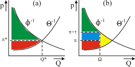
In the formula 2, W is the social welfare, which is a function W(u) of the utility vector uk. The function Φn is equal to the social demand Qn. The individual demand curves qn,k are piled up, as it were. Incidentally, sometimes it is convenient to assume a representative individual, so that all individual demand curves are identical. Thanks to the function Φn(p,W) it can be analyzed to what extent the policy of the state reduces the welfare W. First, consider the common market situation. It is shown in the figure 3a, where in accordance with the common convention the product price is registered along the vertical axis. So in fact this cruve is pn = Φn-1(Qn), where Φ-1 is the inverse of the demand function. The welfare W is constant on Φn.
Next consider the producers. Call the function Qn = Θn(pn) their total supply-curve. The marginal production costs cn are obviously a limiting factor for the size of the supply. The cn are determined by the available equipment (the stock of capital goods), which is bounded. When the available production capacity is overloaded, then cn(Qn) will rise excessively. Then it is also necessary to work overtime, etcetera7. It is often assumed, that one has pn=cn, because thanks to competition on the markets the profits would be negligible. Then the function Θn rises for an increasing pn, because the production costs can increase just like pn. In other words, the social profit is constant on the curve Θn. In the figure 3a the inverse function Θn-1 is shown. The demand and supply are identical at the equilibrium price πn*. In the equilibrium Qn* the markets clear.
Now the total consumer surplus CS can be read from the figure 3a. It is represented by the green area. It can be calculated as
(3) CS(Qn*) = ∫0Q* (Φn-1(Q) − πn*) dQn
The private markets create the consumer surplus, which contributes to the welfare W. This completes the welfare analysis for the consumptive sphere8.
Next consider the situation of the producers. They have costs cn = Θn-1(Q), and these are below the product price πn*. Since the producers can demand πn* on the market, they apparently receive a producer rent PR. The rent is represented by the red area in the figure 3a. It can be calculated by means of an integration, just like the CS in the formula 3. The PR also contributes to the social welfare W 9. Thanks to the private market there is a total social surplus MS, which is the sum of the CS and PR. In other words, the MS is the total of the green and red area in the figure 3a. It can be calculated as
(4) MS(Qn*) = ∫0Q* (Φn-1(Q) − Θn-1(Q)) dQn
The state is indispensable, because a regime must be created, which allows the private markets to prosper. But regimes also coerce, and therefore they lead to discontent and reduce welfare. A state intervention forces the individuals to change their behaviour, and this change often undermines the efficiency. A familiar example is the levying of taxes. They are indispensable, because the state must be paid, but they lead to much annoyance. Thanks to the theory of the social surplus the loss of welfare due to taxes can be depicted. Suppose that the state imposes a consumer tax τn on the acquisition of the product n (VAT, excise, import tariff). This raises the unit price to πn+τn. The demand function Φn(pn) shows, that then the consumed quantity decreases to Ωn. This is shown graphically in the figure 3b.
Thanks to the tax the state receives a sum τn×Ωn. See the blue area in the figure 3b. These benefits are at the cost of the consumers, who must give up a part of their consumer surplus CS for this. The tax does not affect the incomes πn of the producers10. Thus it seems, as though the tax is socially neutral for the welfare W. However, both the CS and PR diminish, because due to the state intervention a quantity Qn* − Ωn of the product n can no longer be sold. The incentive to consume has changed. This lost social welfare is called the dead-weight loss (DWL)11. It corresponds to the yellow area in the figure 3b. It can be calculated with the formula12
(5) DWL(τn) = ∫ΩQ* (Φn-1(Q) − Θn-1(Q)) dQn
So it is important to compare the possible advantages of state interventions with the accompanying lost welfare. In this case the problem is fiscal. Similar problems occur in the income tax, because these actually lower the incomes13. Therefore the incentives to work or to save are attenuated. In principle taxes can be imposed without disturbing the economic behaviour of the individuals, namely when τ is a remittance of money, which is equal for all individuals. This is called a lump-sum, or a poll tax. This is to say, it is independent of economic behaviour, such as consuming or producing. However, the equal lump-sum for everybody can not be reconciled with feelings of justice and fairness. For, such a tax would increase the relative differences in income. The secondary distribution would become more unequal14.
Just now the social welfare function (in short SWF) has been introduced in the argument. A recent column has already discussed the first principles of this SWF. According to the spiritual fathers of this concept, A. Bergson and P.A. Samuelson, the SWF is simply the utility function of the central planning agency. The SWF can represent targets, but also norms and values. Often the SWF is moelled as a general utilitarian function, of the form
(6) W(u) = Σk=1K gk(uk)
In the formula 6, there is a society of K members. The variable uk is the yield of the member k (k=1, ..., K). Strictly speaking this yield is the individual utility of the welfare of k. However, the reader is warned, that some models also interpret uk as purely material benefits. The function gk is the weight, which is attributed to the interest of k by the central planning agency. It has yet to be defined more accurately, but in any case it satisfies ∂gk/∂uk > 0. This condition is self-evident. It guarantees, that the principle of collective growth of income has been satisfied. This is to say, when each individual k receives an additional constant yield Δu, then the social welfare W must increase. Besides, it guarantees that the principle of monotony has been satisfied. This is to say, when an individual k receives more yield Δuk, whereas the other yields remain unchanged, then W must also rise15.
Moreover, the function W of the formula 6 satisfies the principle of strict independence within the society. This is to say, when in a subgroup of society one has W(us) > W(vs) (where the two different utility vectors of the subgroup s are compared: us≠vs), then this order remains unchanged, even when elsewhere in the society the yields change16. Thanks to the weight gk, the SWF can model for instance a policy for target groups. However, for the sake of convenience it is often assumed, that gk = g holds. Then the principle of anonimity is valid, so that no individual k is priviliged. All are mutually exchangeable. In other words, a permutation of the members k does not change the value of W 17.
The social inequality is also important, besides the welfare W. Previously it has been argued in the Gazette, that the choice of the measure μI of inequality is subjective. Then it has already been suggested, that this measure can be coupled to the SWF. The argument is as follows. Suppose that there is indeed anonimity. Then the representative yield ω can be defined by means of the equation g(ω) = W/K. Therefore ω can be calculated from g-1(W/K), where g-1 is the inverse function of g. Define also the average yield as ν = Σk=1K uk/K. Now there are two plausible measures of inequality18
(7a) μIa = g(ν) − g(ω)
(7b) μIb = 1 − ω/ν
These measures of inequality differ, because μIa depends on the total yield K×ν. On the other hand, μIb is based on the ratio of ν and ω, so that the scaling effect of an increasing yield is absent. It is desirable, that the measure of inequality is normalized19. This is to say, one must have μI=0, when uk=ν holds for all k. Moreover one has μI(α×u) = μI(u) for an arbitrary scalar α. So this invariance for scaling does not hold for μIa 20. And finally μI remains unchanged, when the society expands with copies of itself. In other words, each individual k can be interpreted as a group with n members.
The measures μIa and μIb are especially important for the case ∂²g/∂uk² < 0. Such a function g is called concave21. Then the utility of an extra yield Δuk decreases, at least for the society, according as uk is larger. Under this condition SWF W(u) expresses an aversion against inequality22. Thus the desire for levelling is included in the model. This step uses the psychological insight, that unfair inequalities indeed cause discontent with the harmed people. When the SWF attaches a value to the inequality, then it can be represented by W = W(ν, μI, K) 23. So this function takes into account inequality and K×ν, the total unweighed ("material") yield. Now the form of g(uk) is important. Note already now, that the pure utilitarian weight g(uk) = uk does not satisfy inequality aversion. This type of W remains unchanged after a redistribution from the poor to the rich.
The theory of measures μI provides for the insights, which allow to find an appropriate g(uk). For this define two extra principles24. The principle of the transfers states: when yield is transferred from an individual to a richer individual, then the measure μI must indicate, that the distribution of yields has become less equal. Such a transfer does not change the average ν, but it does decrease the representative yield ω. Therefore for instance the value of the measure μIb will increase, because ω/ν decreases. Moreover, introduce a second principle of independence. Namely, in a subgroup s of the society the measure μi(us) must always establish the same order among the various utility distributions us, irrespective of the yields in the rest of the society. Now the four principles of inequality (anonimity, irrelevance of scale, transfers and independence) lead to a unique function of equality25:
(8) f(u, θ) = Σk=1K ukθ
In the derivation of the formula 8 a constant total yield K×ν is assumed. The scalar θ is a parameter, which must not be θ=0 or 1 26. The function f has the property, that it assumes the extreme value (K×νθ) for complete equality uk=ν for all k. Apparently it is not normalized. When θ<1 holds, then other utility distributions are valued higher. Now complete inequality is the minimum of f.
Furthermore the choice of θ determines the specific sensitivity of the function f. For instance, when θ→-∞ holds, then the value of f is determined completely by the smallest uk. More generally, for low values of θ, f attaches the largest weight to the lowest yields uk in the evaluation of inequality. Conversely, for high values of θ (much larger than 1) the evaluation of inequality mainly weighs the largest yields uk. The influence of θ is naturally a problem, because thus there exists an infinite number of measures μI of inequality. The choice of a certain measure is in essence subjective. Everybody could select the measure, which pleases him or her the most. Some will mainly value the utility of the poorest, whereas others attach more weight to the inequality in the middle class. In other words, the choice of θ determines which subgroup is analyzed. With such a flexible measure it is evidently impossible to engage in science!
The function f is actually used in the derivation of a measure μI of inequality. However, a clever find is to base the SWF itself on this function f of equality. A logical choice is g(uk) = β×ukθ, where β is a scalar. Then the SWF equals β×f! The principle of monotony requires, that β depends on θ. In the literature one finds β=θ or β=1/θ 27. When W must express an aversion against inequality, then it must be concave. The choice g(uk) = β×ukθ implies θ<1. Then the welfare indeed increases as a result of levelling. Moreover, this emphasizes the position of the poor. In the extreme case θ→-∞, W even represents the maximin principle of Rawls. Apparently θ characterizes the aversion against inequality. Furthermore, note that the social welfare rises with αθ, when the yields grow with a factor α. The grow clearly satisfies the principle of the collective growth of income.
Choose the utility scaling β=θ. The SWF can also be characterized by calculating the elasticity εuk of its marginal utility ∂W/∂uk 28. It is given by
(9) εuk = ∂²W/∂uk² / (∂W/∂uk / uk)
This elasticity will usually depend on uk. But for the selected W it turns out that one has ∂W/∂uk = ∂g/∂uk = θ×g / uk, and ∂²W/∂uk² = ∂²g/∂uk² = θ×(θ-1) × g/uk². Apparently the elasticity of the marginal utility ∂W/∂uk has the constant value εuk = θ-1. It is negative for θ<1. As a result of an increase of the utility (or the yield in the terms of the present column) uk with 1% the marginal utility of W (the growth of the social welfare) decreases by (θ-1)%, irrespective of the value of uk. Functions with this property have a constant elasticity of substitution, and therefore are called CES functions.
A complication of the selected g function is, that for θ<0 the SWF is negative. Then a complete levelling uk=ν leads to the smallest possible negative value of W, for the concerned total yield. It is more clarifying to use a positive SWF. A good choice is the representative yield ω, which is found after a one-to-one transformation of W 29. One has g(ω) = θ×ωθ = W/K, and from this it follows
(10) ω = (Σk=1K ukθ / K)1/θ
Note that for complete equality uk=ν holds for all k, so that in this point ω assumes the value ν. As long as θ>0, ω is positive for all u≠0. When θ<0, then one has ω=0 as soon as any uk=0. Then the aversion against inequality does not accept, that any individual is without yield30. Furthermore it is interesting to analyze the welfare or the representative yield for various utility distributions, when the total yield is given. Especially the case with K=3 can be shown in a graphical manner31. For, then the distribution u has three dimensions and this can be drawn. Assume for the sake of convenience, that K×ν=1 holds. The budget plane of the society has the form u1 + u2 + u3 = 1. This is shown in red in the figure 4a. There is a complete equality along the "ray" through the origin with direction vector (1, 1, 1). It intersects the budget plane in uk = ν = 1/3.
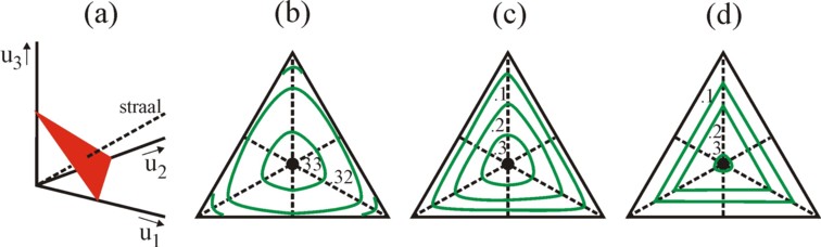
Since the yields are not negative, the budget plane remains restricted to the positive quadrant. Here the budget plane has the form of a triangle with equal sides. In this plane the indifference curves of the representative yield ω are drawn. The figures 4b, c and d show the indifference curves for respectively θ=0.9, θ=-1, and θ=-10 32. In the figure 4b (θ=0.9) there is hardly aversion against inequality. Here ω varies between 0.295 (in the corner points) and 0.333. In the figures 4c-d θ is negative. At the edges of the triangle one always has at least one uk=0, so that there ω=0 holds. The positive indifference curves also have a triangular shape, albeit with rounded corner points. In the figure 4d, ω falls relatively rapidly, according as the distance to the ray of equality increases. Here the indifference curves are mainly determined by the value of the lowest uk. Therefore they are parallel to the edges of the triangle.
Although the figures 4b-c-d present the situation for the total yield 1, they also give an impression of the exchange between equality and the total welfare. Consider for instance in the figure 4c (θ=-1) the indifference curve ω=0.18. On the curve the smallest uk has a value around 1/12 (0.0833), so that both other individuals share the rest with a size of 11/12 (0.917). The same representative yield can also be obtained in a completely equal society (situated on the ray) with ν = ω = 0.18. Here the total yield is merely 0.54, but the poorest individual more than doubles his yield. Apparently the total yield in the society of the figure 4c (with θ=-1) can be halved without punishment, as long as the yields are completely levelled! The reader may decide for himself whether this outcome is realistic33.
Finally the measure of inequality must again be considered. The economist A.B. Atkinson has combined the formulas 7b and 10 in the derivation of his own measure μA. He defines η = 1-θ. Then his measure is
(11) μA = 1 − (Σk=1K ( uk/ν)1-η / K)1/(1-η)
The reader may see, that this measure of Atkinson is based on an elegant theory. Its foundation is a series of well defined principles. The profound analysis is impressive. This is an advantage in comparison with empirical competitors, such as the coefficient G of Gini. Unfortunately μA suffers from the same indefiniteness of the parameter θ (and therefore of η). Moreover, although the theory is indeed elegant, its principles are quite controversial (although certainly reasonable). Policy analists know, that they must not get blinded by the intellectual excellence of models. This all probably explains, why in empirical studies the traditional intuitive measures such as G or the ratio of quantiles are still common, and not μA 34.
The formula 10 for the social welfare uses an interpersonal comparison, where thanks to the parameter θ the importance of the lower yields weighs more heavily in the choice of policy. The economist K. Binmore presents in his book Playing fair (in short PF) another approach for targeted policies35. He states that the social welfare function is given by (p.48, 294 in PF)36
(12) W(u) = Σk=1K αk × uk
The parameters αk are constants. The welfare function W in the formula 12 is purely utilitarian. There clearly is no anonimity. Binmore assumes, that each individual k measures his yield uk by means of his own utility scale, and calls the unit an util (p.54 in PF). The utils of different individuals k are not automatically equal. Now politics must determine the weights, which are attached to the interests of different individuals k. This is done by means of the ratio αm/αn, which values an util of m in utils of n. In other words, αm/αn is a conversion factor or exchange rate of utils. The exchange rate expresses, that an interpersonal comparison is made between the interests of m and n 37.
The Gazette has regularly concluded, that economists have reservations with respect to analyzing interpersonal differences. For, such an analysis requires morals, so that the theory is no longer value-free. However, Binmore makes plausible, that the interpersonal comparison is a common social phenomenon. Namely, life in a group requires, that the individual behaviour must be mutually coordinated. Since the group must be durable and balanced, the members try to avoid conflicts (p.57, 289 in PF). Therefore they are inclined to take into account the ideas and well-being of the others (p.56, 288). They use their capability to show empathy. Empathy furthers cooperation, and therefore Binmore assumes, that it offers an evolutionary advantage (p.58, 297). The capability to show empathy is genetically favoured.
Thanks to empathy it becomes possible to formulate shared preferences (p.290). Social institutions form, as well as collective morals38. Morals are transferred by means of imitation and education (p.65). In the long run the morals naturally adapt to the social changes. The system follows a path of subsequent social equilibria (path dependency). But in the short term the collective morals are fixed. Thus Binmore believes, that a social consensus emerges with regard to the values of the exchange rates αm/αn. This consensus is indispensable for chosing the optimal social order from all conceivable options. This is illustrated in the figure 5.
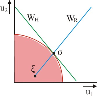
For the sake of convenience the figure 5 is limited to the 2-dimensional case. The red curve defines the area (u1, u2) of possible utility vectors. The outer border of the area is Pareto optimal. The social optimum must be selected somewhere on the Pareto border. Commonly the point is chosen, where the welfare line W(u) of the formula 12 touches the set of possible utility vectors. The figure 5 shows the welfare line in green. Binmore attributes this welfare line WH to the economist Harsanyi. However, this W is neutral with respect to inequality. Therefore the citizens will also demand, that the maximin principle of the philosopher Rawls is satisfied.
This principle usually has a different optimum than pure utilitarianism. Namely, suppose that the minimal allowable yield of the individuals k=1 and 2 is given by ξ = (ξ1, ξ2) (p.48). This point defines the origin of the utility scale, and is shown in the figure 5. Since also here the utils of the individuals differ, and must be converted, the welfare function WR according to Rawls equals
(13) W(u) = minimim van (α1 × (u1 − ξ1), α2 × (u2 − ξ2))
Next the maximum of this minimal welfare WR must be selected. In other words, none of these two values must be less than the other. So the maximum must lie on the line α1 × (u1−ξ1) = α2 × (u2−ξ2). This line is shown in blue in the figure 5. Now the find of Binmore is, that thanks to the empathy of the citizens the values α1 and α2 are chosen in such a way, that the optima of WH and WR exactly coincide on the Pareto border, in the point σ (p.88)39. Thus Binmore presents an alternative way to model the aversion against inequality. He assumes, that the citizens together distinguish between apparent social groups and their interests. On the other hand, the approach with the parameter θ of inequality assumes, that low yields naturally obtain more weight. Then the mechanism of empathy, which leads to shared preferences, remains invisible40.