The distribution of incomes

First insertion on Heterodox Gazette Sam de Wolff: 15 may 2018

Until now the Gazette has not paid much attention to the theory of income distribution. However, this theory is indispensable in the analysis of the welfare state. Therefore the present column discusses the main principles. The difference between gross and nett incomes is explained. Various pictures of the income inequality are shown, such as the frequency distribution and the Lorenz diagram. Several common measures of income inequality are described, among others the parameter of Pareto and the Gini coefficient.

More than five years ago the then chairman Spekman of the PvdA made the surprising remark: "The levelling of incomes is a joy!" His remark caused so much hilarity, that "levelling party" was almost chosen as the expression of the year 2012. The reality is evidently more complex, and the present column wants to give some insights into the optimal and fair distribution of incomes¹. This is an elaboration of a long series of articles, which study various income aspects. Sam de Wolff, the name-giver of the Gazette, shows that the disutility of work must be compensated by a reward. A column from 2013 describes how the Belgian politician Hendrik de Man summarizes the various factors, which contribute to the displeasure of work. Moreover, he shows that the reward partially consists of non-monetary factors.

In the same year a column appeared, which discusses the compensating wage differences. Workers choose their job not purely on the basis of the wage, but they also take into account the secondary job conditions. During the sixties the Dutch economist Jan Tinbergen presented this phenomenon as a theory of tension. According as the job demands s_n deviate more from the properties t_n of the worker, his disutility of work will increase. When the worker is under-qualified (say, t_n < s_n), then he will probably be compensated with a relatively high wage². A year ago all these models have been summarized again in a separate column. Here the following formula is takes as the starting point:³

(1)     u(e, w) = v(w) − c(e)

Figure 1: Quartet card
   catholic youth work

In the formula 1, u is the utility (job satisfaction) of the worker. It is composed of two parts, namely the pleasure v(w) due to the wage w, and the displeasure (costs) c due to the effort e. An important goal of such models is evidently to justify the really paid money wages w. Whenever possible, Tinbergen wants to establish work classifications, and calculate from them the corresponding wage w. The Dutch economist Bernard van Praag has determined empirically, how the various factors at work contribute to the satisfaction u of the job. It turns out that the job contents is more important for u than the wage height⁴. Van Praag succeeds in measuring the preferences of the average or representative worker, and therefore describes the relation with the macro level of the economy.

Already in 2013 a column discussed the study by Jacob van der Wijk, a friend of De Wolff, who indeed analyzes the income distribution at the macro level. Van der Wijk elaborates on the spread of the incomes, as well as the effects of inequality on the wellbeing of individuals. Since this is an analysis at the macro level, Van der Wijk can not take into account various factors, which compensate the inequality in incomes. Here one identifies also the evident logical error in the cited remark of Spekman. This makes his statement unfair. For, the differences in money wages, are mainly caused by free choices. The individual chooses his own education, working hours, industrial sector, or composition of the household. Those who want to judge the justice or fairness of wage differences, must take this into account. The present column wants to elaborate on such considerations. Therefore the formula 1 is rewritten as⁵

(2)     u(w, a) = v(w) + ω(a)

In the formula 2, a represents the labour conditions, with the exception of the wage w, and ω(a) is the total utility, which these labour conditions yield. So the formula 2 separates the rewards in money from the immaterial rewards. Many economists believe, that the fairness of society must be tested against the levelling of u(w, a) (so not of w)⁶. However, here it must be remembered, that the state has many goals, which are at least as important as fairness or justice. The state must realze all of these goals in the best possible manner, with a fit weighing factor for each goal, and therefore tries to realize the optimal income distribution⁷. In spite of many attempts to measure ω(a), this term remains quite speculative. Therefore the economic science has yet mainly studied the income distribution, so the incomes w_k of all K citizens or households.

The incomes

The introduction of this column actually only considers incomes from labour. However, it is common that a part of the individual income is not related to labour. It consists of for instance interest, or (house) rent, thanks to the property of respectively capital, land, or real estate. The profit of the entrepreneur also is an income, due to labour or not⁸. All of these incomes are rewards for production factors. The rewards express the scarcity of these factors on their respective markets. The incomes on the factor markets are not yet taxed. These are called the primary incomes, in short YP. However, these incomes are not freely available for the receivers. For, the state must also be paid, and he obtains his financial means by imposing taxes on the private incomes. Moreover, the individuals are obliged to pay premiums for the various employee- and employer-insurances.

Figure 2: Quartet NVM

So the state reduces YP by means of his direct income taxes. On the other hand, the state sometimes also increases the incomes, by means of transfers such as subsidies and benefits. The direct taxes and the transfers determine together, what the really available income of the individual is. The available income is called the secondary income, in short YS. Since mainly the poor individuals qualify for benefits, the distribution of YS is somewhat more equal than the distribution of YP. Although YS is completely available to the individual, this does not yet finalize the state intervention. Namely the state also imposes indirect taxes, on consumption. Consider the VAT (tax on added value), excise duties (taxes on alcohol etcetera) and import levying. Some believe, that the indirect taxes lead to a greater inequality. Namely, it does not effect the savings⁹.

So strictly speaking the income must be corrected for the effects of indirect taxes, notably when one is interested in inequality (differences in really available incomes). Furthermore, the state uses a part of its financial means for supplying public goods and services, which are consumed in kind, such as education, health care and culture. They are immaterial benefits of the type ω(a) for the users. Collective goods such as defence and justice can also be included in the individual benefits. According to the formula 2 such benefits must be added to the individual income. When the secondary income is corrected for the effects of indirect taxes and of the individually consumed public facilities, then the so-called tertiary income is found, in short YT. State interventions guide society, and therefore also change YP¹⁰.

Until now the focus is on the individual income. However, individuals often live in households, which consist of a number of persons f. These f individuals together will share the income of the household. Here they profit from advantages of scale, because many domestic appliances can be mutually shared. Consider the television set, heating, books, clocks, to a lesser extent also the washing machine and the car, etcetera. A child consumes less than an adult. Thus a false impression could be created, when the individual income is calculated simply by dividing the aggregate income of the household by f. Nowadays the European Union and the OECD both use an equivalence scale for adults, which within the household weighs each extra adult by 0.5, and each child by 0.3. In other words, in a household with n adults and m children f is corrected by means of f' = 1 + (n−1) × 0.5 + m×0.3 ¹¹.

Dependent on the theme, analyses study the incomes per individual or per (member of the) household. Such incomes are called personal. It has just been remarked, that an individual or household can own various production factors. The interest of economists is strongly focused on the incomes of these factors. The income of a factor is called functional, because each factor has its own function within the production process, In the present column the focus is on the personal distribution, and the functional distribution is merely of an incidental importance¹².

The income distribution

The analysis of the distribution of incomes gives insight in the fairness of society. Suppose that the society consists of N individuals (or households). Let y_n be the personal income of the individual n (with n=1, ..., N). Reorder the individuals into a row with increasing y_n. Then one finds the curve, which is shown in the figure 3a. Each n on the horizontal axis is coupled to a "bar", which is as high as his income y_n. This is called the procession of Pen¹³. For comparison, the figure 3a also shows the average income y_g per individual. The procession is naturally discrete in n, but it is mathematically convenient to approach the distribution y₁ ≤ y₂ ≤ ... ≤ y_N by a continuous function y(n). Moreover, the size N of the population is irrelevant, so that n can be normalized on N without loss of information. So suppose, that Ω=n/N can assume all values between 0 and 1. Then y = P(Ω) holds, where P is the Pen curve in the figure 3a.

Figure 3: Income distribution y(n):
    (a) procession of Pen; (b) cumulative distribution; (c) frequency distribution
        y_g = average income;    y_m = modus income

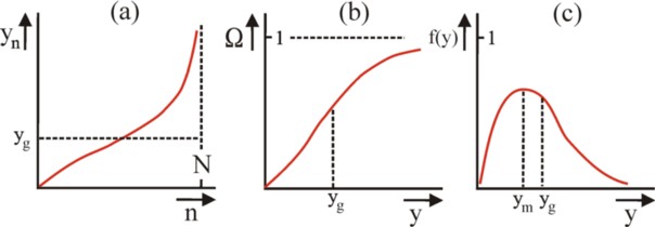
Now the frequency- or probability-distribution of the incomes can simply be derived from P. For, Ω = P^-1(y) holds, where P^-1 is the inverse function of P. It is shown in the figure 3b. Actually the axes in the figure 3a have simply been interchanged (and n is normalized into Ω). Since Ω increases vertically from 0 to 1, the function P^-1(y) can be interpreted as the cumulative distribution function of the incomes y. Therefore f(y) = ∂P^-1/∂y is the frequency distribution (density function) of y. See the figure 3c. It is skewed. In other words, the most often occurring income y_m (the modus) is less than the average income y_g. This will not surprise the loyal reader, For, a previous column explains, that according to the sociological thinker J. van der Wijk y = μ + e^u/κ holds, where μ and κ are constants, and u is a Gaussian distribution around zero. This causes a long "tail" of high incomes.

A more interesting aspect of the row of Pen (y = P(Ω)) is, that it allows to simply construct the so-called Lorenz diagram. For this purpose, define the cumulated income Y(n) as the summation of the incomes of all individuals between 0 and n in the figure 3a. This is to say, Y(n) = ∫₀ⁿ y(ν) dν= ∫₀^Ω×N y(ν) dν = N × ∫₀^Ω y(ξ) dξ = N × ∫₀^Ω P(ξ) dξ. For n=N this is dit a summation over all individuals N, so that Y(N) = N×y_g equals the total income of society. Define the normalized cumulated income as Ψ(Ω) = Y(n) / Y(N) = Y(N×Ω) / Y(N), so that Ψ varies between 0 and 1, just like Ω itself. Then Ψ(Ω) is the so-called Lorenz curve. She is shown in red in the figure 4, for the row of Pen in the figure 3a.

Figure 4: Lorenz diagram:
    for figure 3a, equality,
    and maximal inequality

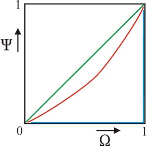
The Lorenz diagram presents the inequality in a peculiar way. For complete equality one has y_g = P(Ω), so that Ψ(Ω) = Ω must hold. Then apparently the Lorenz curve is the green diagonal in the figure 4. In maximal inequality the individual N owns the total income Y(N). This can mathematically be represented as a delta function, namely P(Ω) = Y(N) × δ(Ω−1). Now the Lorenz kromme curve follows the blue trajectory (Ω, Ψ) = (0,0) - (1,0) - (1,1) in the figure 4. All other Lorenz curves lie between the green and blue extreme situations. Finally, note that the Lorenz diagram, and incidentally als the figures 3a-c, can be constructed for the primary and secondary incomes, as well as for individuals and households.

Measures of inequality

The previous paragraph has discussed various ways to depict the income distribution. However, such pictures merely present a qualitative comparison between the various distributions. Quantitative comparisons are more clarifying, and therefore, for a long time science has tried to find convenient indicators (measures) of inequality. Besides, there is obviously the hope, that the analysis of distributions will lead to a sound economic theory. Unfortunately, until now this hope is idle, because an all encompassing model is still missing. One must be contented with semi-empirical models, which moreover only describe a part of the distribution¹⁴.

Quantiles

An evident approach is to strongly compress the frequency distribution. For, it is impossible to compare all personal incomes y_n (with n=1, ..., N) with each other. Therefore an empirical analysis will always restrict itself to the distribution over groups. This inevitably destroys information. This is particularly clear in the computation of the average income, which makes the distribution invisible. Commonly, the separate incomes are aggregated (collected) in quantiles. This is to say, first the personal incomes are ordered according to increasing incomes (row of Pen). Subsequently this row is split into Q groups (with N/Q members each). The income φ(q) per group q is determined by φ(q) = Σ_n=j+1^j+N/Q   y_n, where j = (q−1) × N/Q. Finally, each quantile is also normalized, with Φ(q) = φ(q) / Y(N). The cases Q=4, 5, 10 and 100 are called respectively a quartile, quintile, decile and percentile.

Therefore the first quantile (q=1) unites the N/Q lowest incomes, and the last (q=Q) quantile unites the N/Q highest. Those who want to study poverty, will analyze mainly q=1. When the quartiles are preferred. then q=2 and 3 represent the lower and higher middle classes. The continuous row of Pen P(Ω) has changed into a discrete bar graph Φ(q).

The α measure of Pareto

The well-known economist V. Pareto believes, that the distribution is characterized by a single parameter α. For this reason he considers the variable R(y) = ∫_y^∞  f(η) dη. By definition this cumulative function equals R(y) = 1 − P^-1(y). Apparently this curve is the figure 3b on its head. Pareto supposes, that the tail of R(y) (so the higher incomes) is described by R(y) = c / (y − d)^α. Here c is a scaling factor, and d is a lower threshold of y. Obviously the problem of this model is, that due to the threshold the lowest incomes are not taken into account. The model is mainly useful for the analysis of the higher incomes. Besides, the measure α does not give a theoretical explanation¹⁵.

The coefficient of Gini

The coefficient of Gini (G) is a popular measure for the inequality of the distribution. G is defined by means of the Lorenz diagram. Namely, G is simply twice the surface between the diagonal and the Lorenz curve in the figure 4. Thanks to the multiplication by 2, G has values between 0 (for an egalitarian distribution y_n=y_g) and 1 (for total inequality y_N = N×y_g). Unfortunately, there is no clear theoretical interpretation connected to G. Your columnist has also found two formulas for computing G¹⁶. The first one is

(3)     G = (2 × N² × y_g)^-1 × Σ_n=1^N Σ_k=1^N  |y_n − y_k|

The second one is, with y₁ ≤ y₂ ≤ ... ≤ y_N,

(4)     G = 1 + 1/N − 2 × (N² × y_g)^-1 × Σ_n=1^N (N − n + 1) × y_n

The measure of inequality of Atkinson

The economist A.B. Atkinson has invented the A measure of inequality¹⁷. A is calculated by forming groups of individuals or households, similar to quantiles. However, now the various groups are not all equally large. This is to say, the group q has n_q member, with evidently Σ_q=1^Q  n_q = N. The definition is

(5)     A = 1 − ( Σ_q=1^Q  n_q × (Y(q) / (n_q×y_g))^1-ε )^1/(1-ε)

Note that one always has A=0 for a completely egalitarian distribution. In the formula 5, ε is the parameter of inequality avoidance. The goal of this parameter is to base the measure of inequality on the social morals. For ε=0 the society believes that inequality is irrelevant. Therefore, in this situation A=0 holds, irrespective of the distribution. According as ε becomes larger, then A will also increase for a given distribution. It seems that A can indeed be derived from a social welfare function¹⁸. Therefore the A measure has a theoretical meaning. Atkinson uses in his model individual utility functions of the form u(y_n) = y_n^1-ε / (1 − ε) ¹⁹. This is a fascinating matter, which will undoubtedly yet be elaborated in the Gazette.

1. Nonetheless, Spekman has probably reinforced his position within the PvdA by his remark. The party members are aging, so that a significant part of the members was formed during the heydays of party leader Den Uyl. At the time the party doctrin is the "spread of knowledge, power and income", so that levelling is natural for the aged members. The doctrin in itself is sympathetic, but since the seventies it is interpreted in a dogmatic and sometimes tyrannical manner. Those who have not personally experienced the period 1966-1977, will probably fail to understand the sometimes bizarre ideas and excesses. Your columnist has known Spekman for a fairly long time, since his period as an alderman, so that this colourful figure is a reference point. (back)
2. The expression of tension theory can be found on p.113 in Naar een rechtvaardiger inkomensverdeling (1977, Uitgeversmaatschappij Agon/Elsevier) by J. Pen and J. Tinbergen. In the modern literature the model of Tinbergen is rarely mentioned. On p.79-81 in Theorie der Einkommensverteilung (1975, Springer-Verlag) G. Blümle does discuss the tension model. Blümle objects, that the market demand of skills s_n will naturally adapt to the present supply t_n (p.80). Moreover, he states on p.81: "Insgesamt jedoch läßt sich die Einkommensgleichheit sicherlich nicht als Kompensation für unterschiedliches Arbeitsleid erklären". Since your columnist is an enthusiastic adherent of the formula 1 and of the hedonistic wage theory, he rejects the criticism of Blümle. For the sake of completeness, an additional criticism of Blümle is also mentioned. Tinbergen assumes, that the individual skills (or the education) are distributed normally over the population. Blümle states on p.80, that this type of skills is learned. Some individuals are excellent pupils, so that the distribution is skewed due to a "tail" of excellence. In other words, learned properties are commonly not distributed in a normal manner, contrary to innate properties. Perhaps this criticism is justified. But Tinbergen develops an empirical model, and then (sometimes crude) simplifications are unavoidable.
   Incidentally, your columnist bought Naar een rechtvaardiger inkomensverdeling from the Utrecht library, when it sold out its stored stocks. He read it fifteen years ago for the first time, and then struggled with the strange mix of complex calculations and superficial phrases. In this way Pen and Tinbergen hoped to address a wide audience. They are part of the generation, which energetically tried to elevate the population, together with among others Arnold Heertje. Nowadays the Dutch economists are more modest in this regard. Pen and especially Tinbergen, both social-democrats, have their main successes during the sixties. After the seventies economics rejects both centrale planning and Keynesianism. Then the authors have difficulties in adapting to the new ideas. The quality of Naar een rechtvaardiger inkomensverdeling suffers somewhat from this rigidity. Moreover, Pen and Tinbergen refer in the contents of this book quite often to norms (morals). They advocate a radical way of levelling, which reminds of Spekman. For instance, the low well-being of handicapped must be compensated with money! (p.66, 182, 198) Whenever possible, long-term unemployed and fragile old people must also be compensated! On the other hand, natural talent must actually be taxed (p.192). Since they acknowledge, that inequality of incomes originates from scarcity on the market, the state must correct this energetically. Therefore a campaign, aimed at changing the mentality, is necessary (p.184). But such coercion fits poorly in the present time of regained liberalism. It is rather tactless. that they sometimes include political slogans in their text. For instance on p.118: "We agree with their practical conclusion that the United States would benefit from a social-democratic movement". Or on p.202: "Their parents [of the youth] watch television, completely manipulated". Pen would finally end as a columnist for, among others Vrij Nederland, where he wrote rather rancorous texts. (back)
3. In 2015 a column has appeared, which considers the wage as a compensation for the forgone leisure time t_v. Then u = v(w) + ν(t_v) holds, where ν is the utility of leisure time. Note that an increase of t_v equals a decrease of the effort e. The formula 1 implies, that the displeasure of work and the costs c of effort are compensated by the wage w. On p.197 in Naar een rechtvaardiger inkomensverdeling Tinbergen promotes this view, whereas his co-author Pen argues, that a higher wage w is accompanied by lower personal costs. The contents of important jobs would be pleasant. Blümle supports Pen on p.81 in Theorie der Einkommensverteilung: "Einkommen, Ansehen, Einfluß und Erfüllung bei der Beschäftigung sind positiv korreliert". Here your columnist supports the view of Tinbergen, without reservations. Important jobs correspond to huge responsibilities, for instance with regard to self-motivation. This is a heavy burden. Only a masochist or sadist would be pleased by a restructuring or austerity in the division of a company. (back)
4. This probably means, that the employers pay a satisfying wage to their workers. The wage conforms to the social standard, and is experienced by the worker as natural. On p.110 and further in Naar een rechtvaardiger inkomensverdeling it is mentioned, that Tinbergen and Van Praag have cooperated in 1976. Fifteen years ago, when your columnist read this book, he did not yet understand the significance of the method of Van Praag. This became apparent only ten years later. (back)
5. This formula is taken from p.122 in Economics of the welfare state (2004, Oxford University Press) by N. Barr. Barr calls this the complete income. Barr does not express clearly, whether the complete income is expressed in money, or in units of utility. Your columnist prefers to use utility functions. When the utility of money is known, then each variable can obviously be simply calculated from the other. (back)
6. Pen and Tinbergen defend this standpoint in Naar een rechtvaardiger inkomensverdeling, on p.60 and further, as well as on p.104 and further. Incidentally, here they interpret u(w, a) as the average utility within certain categories of individuals, such as professional groups. Then u(w, a) does not refer to the separate individual, with all his peculiarities. The Belgian-Flemish economist H. Deleeck pleads on p.33 in De architectuur van de welvaartsstaat opnieuw bekeken (2003, Uitgeverij Acco) in favour of a system, where "the needs of all citizens can be satisfied equally". Barr also wants to level u(w, a) on p.122 and 135 in Economics of the welfare state. However, he believes that the immaterial utility ω(a) can not be measured, and restricts his discussion to the study of the income distribution w. In the column about the study of Van der Wijk it is remarked, that the total levelling leads to u_k(w, a) = β for all citizens k. When the social welfare function W is utilitarian, with equal weights for all K citizens, then it has the value W = K×β. (back)
7. See p.66 and further, as well as p.107 and further in Naar een rechtvaardiger inkomensverdeling. (back)
8. Although the jobless incomes do not equire an effort e, they also aim to compensate a certain displeasure. The beneficiary still has costs c. For, the owner himself can temporarily not dispose of the production factor. (back)
9. The idea is that poorer people consume a larger part of their disposable income then the more wealthy people. On p.24 in Theorie der Einkommensverteilung it is stated, that due to the differences between the national indirect taxes the secondary income distribution is not very suited for making international comparisons of the inequality of the distribution. (back)
10. This profound remark is made on p.33 in De architectuur van de welvaartsstaat opnieuw bekeken. The welfare state changes the human behaviour (p.72). Blümle notes on p.14 in Theorie der Einkommensverteilung, that individuals and groups sometimes succeed in shifting the consequences of state interventions (taxes, payment of premiums) to their clients. However, the present column does not aim to analyze the finances of the state. In the future the Gazette will undoubtedly discuss finance. According to p.374 in Économie politique de la protection sociale (2011, Presses Universitaires de France) by M. Elbaum it is difficult to calculate YS and YT exactly, because the state interventions are so fragmented. They are spread over the various policy domains, but also across the administrative layers (state, province, municipality). (back)
11. See p.298 in De architectuur van de welvaartsstaat opnieuw bekeken. Deleeck argues on p.298, that YT is the best measure for welfare. (back)
12. On p.295 in De architectuur van de welvaartsstaat opnieuw bekeken it is remarked, that incomes can also be ordered in categories, such as young and old, or men and women, or various nationalities. Such analyses use both economics and sociology. This way of ordering is irrelevant for the present column. On p.3-4 in Theorie der Einkommensverteilung the functional distribution is coupled to the neoclassical paradigm. (back)
13. See p.17 in Naar een rechtvaardiger inkomensverdeling. The row of Pen has gained some popularity, although it does not give much extra insight in comparison with the frequency distribution n = f(y). (back)
14. The theories of the quantiles, the α parameter of Pareto, the Lorenz diagram and the Gini coefficient G are all more than a century old. Jacob van der Wijk discusses them in detail in his book Inkomens- en vermogens-verdeling (1939, De Erven F. Bohn N.V.). In the past century attempts to find better measures of inequality have failed (perhaps with the exception of the A measure of Atkinson). Obviously since analysts did succeed in accumulating an enormous amount of statistical material. In addition the distribution of incomes has become more complex. Nowadays the social security affects the YS, for instance by paying pensions. Naar een rechtvaardiger inkomensverdeling points on p.18 en 60 to the fact, that the state pensions are in the lowest income categories. However, before the Second Worldwar such pensions hardly existed, so that they did not enter in the individual YS. This reduces the degree of inequality. Nonetheless, these pensions do improve the welfare of the old people.
    Several criteria can be formulated for a measure of inequality. On p.37 in Theorie der Einkommensverteilung the condition of Pigou-Dalton is mentioned: in an income transfer from a rich person to a poor person the measure must express an increased levelling. The condition of Bresciani-Turroni is: a proportional rise of all incomes must not lead to a change in the value of the measure (p.38). (back)
15. It is worth mentioning that ∂R/∂y = -∂P^-1/∂y = -f(y) holds. Considering the supposed functional form of R one also has ∂R/∂y = -R×α / (y−d). In other words, R(y)×α = (y−d) × f(y) holds. Apparently the R-function gives an extra weight to the high incomes in the tail of the frequency distribution f. The distribution f(y) falls even faster than R(y), which makes sense, considering its form in the figure 3c.
    Van der Wijk derives on p.266 and further in Inkomens- en vermogens-verdeling relations between R(y) and his own formula u(y) = ln(y−m). Here the utility of income u(y) has a normal distribution, with standard deviation σ. In this manner he derives α + 1 = (2×σ²×u + 1) × (y−d) / (y−m). So, according to Van der Wijk the α parameter of Pareto is not a constant, but depends on the income y. Since α is mainly relevant for high incomes y, this relation can be approximated by α = 2×σ²×u (p.269). Now Van der Wijk proposes to restrict the analysis to high incomes, with u>0. Then on average one has u_g = (σ×√π)^-1. It follows from this that α_g = 2×σ/√π = 1.13×σ. On p.210 Van der Wijk states, that this formula conflicts with the statistical data. However, empirically α/σ = constant does hold approximately. In this manner Van der Wijk yet gives a theoretical meaning to the α parameter of Pareto.
    According to Van der Wijk the income distribution is purely stochastic. This is to say, two incomes y_a and y_b are always totally uncorrelated. In practice this is of course not true. Blümle gives in chapter 2 of Theorie der Einkommensverteilung various possible explanations for the log-normal distribution of incomes for labour, in the paragraphs 2.1-2.5. In paragraph 2.6 of chapter 2 the incomes of capital are studied. Incomes of labour are an interesting matter, and it turns out that the methodological individualism is useful. For, it it logical to couple the personal income to certain personal skills. Even when skills within the population have a normal distribution, then the skills of an individual can yet reinforce each other. This can lead to high incomes. Hierarchical (organization-) structures also affect the individual incomes. The so-called human capital school explains the personal income by means of the received education (just like Tinbergen, albeit with another argument). In this model, education is an investment, which raises the income in the later professional life. In fact here the formula 1 is applied, where e is the duration of the education. In a variant of this model it is assumed, that the received education serves as a signal on the labour market. It is strange that Blümle does not like this approach. On p.62 he writes: "Die konsumtiven Aspekte [der individuellen Bildungsausgaben], die oft mit dem Schlagwort Lebensqualität angesprochen werden, bleiben unberücksichtigt". And on p.65: "Die der Theorie zugrunde liegenden Investitionskriterien können sicherlich die durch Neigung intuitiv und durch Herkunft gesellschaftlich bestimmte Entscheidung der Individuen hinsichtlich ihrer Ausbildung kaum ausreichend beschreiben". And on p.168 in Naar een rechtvaardiger inkomensverdeling it is stated, that the theory of the human capital fails to address "the human ambition to unfold oneself. ... This view contradicts the humanistic view on education". Your columnist does not support this criticism. It is unwise to believe everything, that is published. Individual decisions are certainly complex, but students do realize, that they invest in their future. Quite a lot of students are not internally motivated by the spiritual wealth of knowledge. Thinkers such as Paul Frijters, James Coleman and Ken Binmore rightly believe in the homo economicus as a model of human behaviour. (back)
16. The first formula can be found on p.101 of Economic inequality and income distribution (1998, Cambridge Unitersity Press) by D.G. Champernowne and F.A. Cowell. The second formula can be found on p.142 of Economics of the welfare state. The first formula is apparently a discrete integration of the area in the Lorenz diagram. The second formula can undoubtedly be simply derived from the first one, but your columnist has not tried to do this. On p.302 in De architectuur van de welvaartsstaat opnieuw bekeken the second formula is presented in the form G = 2 × (N² × y_g)^-1 × Σ_n=1^N (n − ½ × (N + 1)) × y_n. On p.43-45 of Theorie der Einkommensverteilung the Gini coefficient is calculated for several simple but illustrative examples. (back)
17. See p.144 in Economics of the welfare state. (back)
18. See again p.144 in Economics of the welfare state. (back)
19. See p.127 in Economics of the welfare state. Loyal readers recognize this function from a previous column, which discusses the CPB report Distributionally Weighted Cost-Benefit Analysis (2017). There the parameter ε of inequality aversion is represented by the symbol μ. (back)