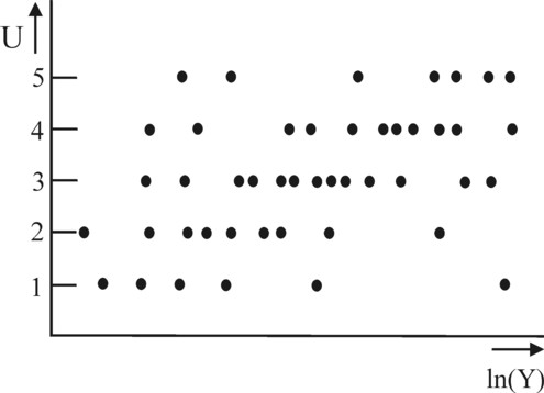
Figure 1: Measured values of U and ln(Y)
At the moment this portal has already placed many columns concerning measures for utility, and related variables such as preferences and satisfaction. A measurement requires a scale. The present column studies the scaling methods, which are used in the science of sociology. In the general discussion the methodological frame is introduced, including some excursions to Leninist works (with thanks to the second-hand bookstore Helle Panke). Next the Probit method is explained, in the form that Bernard van Praag applies to the scaling of the utility for monetary incomes.
The human sciences differ from the natural sciences by the character of the object, that is studied. For instance the sociology analyses the human attitude, that is to say the various types of behaviour and opinions, in a social context1. The knowledge about this theme is also required in economics, as far as it concerns subjective choices, such as human preferences. A researcher will investigate a certain aspect of the human attitude, and will try to increase the empirical and theoretical knowledge. The collected empirical data are usually transformed in such a manner, that they can be presented as one or more indicators. Thus the information, which is available in the data, can be reproduced succinctly. The focus is on causal relations.
An indicator is objective, when he is constructed from factual data (numbers, formal types, material observations, etcetera). An indicator is subjective, when he is composed of personal opinions. The only requirement on the form of the indicator is, that he contains information about the studied aspect of the human attitude. A common example of the indicator is the index (itself composed of various indices, such as the human development index).
The numerical value of the indicator is found by performing various measurements within the target group of the study. The attachment of a value to the indicator requires the presence of a measuring-scale. In sociology it is often attempted to determine the consciousness within the group with regard to an aspect or subject. A popular method to measure the value of an indicator is the questionnaire, where each question pertains to a certain item. Each item has its own scale. The present column discusses the income satisfaction, and she can be measured by a single question (item).
Measurements must be objective, that is to say, they lead to the same result, irrespective of the researcher. Furthermore they must be reliable, and thus reproducible in a repeated measurement. And finally the measuring-method must be valid, that is to say, it gives a meaningful result. This last point can for instance be tested by means of a theoretical model (construction). Suppose that the theoretical model yields the value X, then the measured value will be Y = X + ε, where ε represents the deviation. The deviation must not be systematic, because then the measuring-method (or the model) is not sound. Therefore the expected value E[ε] of ε must equate zero, when a large number of measurements is performed2.
The theoretical construction is called the latent dimension, because she can not be observed directly. Sometimes the model is multi-dimensional, and employs for instance n quantities Xj (j=1, ..., n). In such a factor-analytical model the measured value satisfies Y = (α·X) + ε. Here X is the vector notation of Xj and α is a vector of constants, whose values are chosen in such a way, that the identity with Y is optimized. This process of approximation is called a fit. The term in brackets represents the algebraic inner product.
On this portal the previous columns about the economic utility often distinguish between an ordinal scale and a cardinal scale. For a long time economics has argued that the use of the cardinal scale is controversial. The economist V. Pareto began this controversy, when he showed that sometimes the theory needs merely the ordinal scale. Therefore the use of the cardinal scale is superfluous3. Indeed the cardinal scale is more concrete than the ordinal scale. But this also implies, that it contains more information. Often this extra information is important, so that still the cardinal scale is preferable. In economics the support for this approach grows, according as more inter-disciplinary studies appear.
The sociology disposes of an extensive classification of scaling methods. It is worth while to discuss them, because that adds to the insight. The simplest scale is nominal. Here the measured value is simply a grouping in categories. For instance: sport, gardening and reading are categories of leisure time activities. Any grouping is acceptable, as long as they distinguish between categories. The number of meaningful mathematical operations is limited, for instance determine the class or set with the largest number of elements.
In the ordinal scale the measurement classifies the objects according to a certain property. The reader is already familiar with the economic example of the individual utility of a product. Here all scales are usable, which classify the objects in the same order. In other words, each transformation of the scale, which leaves the order unchanged, is allowed. The scale is univocal, apart from this type of transformation. A typical mathematical operation on an ordinal scale is the determination of the middle object in a row. The economic counterpart is the cardinal scale, which in the sociology is commonly called the interval scale. This scale contains more information than the ordinal one, and thus it is more concrete.
In the interval scale the distance between all objects is measured, in addition to the order. It is possible to compare two values, which represent differences. A well-known example in economics is the marginal utility, which is computed as the difference of two utility values. The hallmark of this scale is, that it can be transformed by means of a linear transformation, without any loss of information. When on one scale the value X is measured, then the scale with values Y = α1×X + α2 is also satisfactory. A familiar example is the temperature, measured on the Celsius and Fahrenheit scales. Note, that the point zero (origin) does not influence the distances between objects. Here a typical mathematical operation is the computation of arithmetical averages. For they are in essence invariant for transformations: the points with the largest deviations from the average will maintain this property after a linear transformation.
Finally the ratio scale is worth mentioning. Here all ratios of the object values are determined. Therefore the scale really measures percentages. It is clear, that economics is replete with this type of scales: consider the growth rate, the interest rate, the unemployment percentage, inflation, etcetera. The choice of the point zero on the ratio scale is crucial. This is evidently obvious for monetary sums, such as incomes and wealth. Merely the proportional transformations Y = α×X leave the properties invariant. In this scale also the geometrical average is relevant (because it is conserved by proportional transformations).
An interesting hallmark of all these scales is, that the type of scale in a measurement can be determined empirically. It must be checked, whether the measured values satisfy the axioms, which pertain to a certain manner of scaling. For instance, the ordinal scale must satisfy the i>transitivity-axiom. This axiom states, that all measured values yj must satisfy causal relations in pairs: when (yi > yj) and (yj > > k), then one has (yi > yk). It is straightforward to check in an empirical manner, whether indeed this axiom is satisfied. Small deviations can be tolerated, provided that they fall within the margin of error of the measured values.
The loyal reader will not be surprised, that the Leninist professional literature is consulted for additional insights. Little has been found by your columnist. Apparently (and surprisingly) in the Leninist states the sociological research was started forty years later than in the west4. Therefore the Leninist sociologists simply copy the western insights. Now a hallmark (and a curse) of Leninist scientists is their addiction to polemics with regard to anything of a capitalist origin. So the sociologists can not refrain from long lists of reservations, which will be omitted here.
Their most interesting contribution is the idea, that the human conscience must be interpreted according to the Leninist materialism. That is to say, in the end all social behaviour can be connected to the productive relations. This is especially true for the conscience, since this is formed in the process of the material production, and conversely influences that production. Thus the sociology is placed in a materialistic framework, which is absent in the west. The analysis of the human attitude with respect to labour is the spearhead in the Leninist sociology. It is more a limitation than an enrichment.
An advantage is, that this preference focuses the attention of all sociologists on this single theme. They do not have to waste their energy on, for instance, the human perception of yogurt deserts, like in capitalism. Moreover the Leninist paradigm of the historical materialism points out the desired direction of the future developments of the productive structure. In this way it is to a degree possible to judge the desirability of certain human attitudes. Therefore the Leninist sociologists tend to moralize more than their capitalist colleagues, who lack this type of insights. The object of study, the common man, is confronted with a warning sociological finger5.
The theme of the present column is the scaling of the utility of monetary incomes. In the seventies the so-called Leyden school presented a break-through in the knowledge of such utility measurements. The theoretical framework can be found, among others, in chapter 2 of the fascinating book Happiness quantified, by Bernard van Praag en Ada Ferrer-i-Carbonell. Here an effort will be made to explain their arguments in a clear manner. The so-called probit method plays a central role. In order to better understand this method, your columnist has consulted several texts on the world wide web, in addition to the book.
In the last paragraph it is mentioned, that the measurement of the utility of the monetary income poses just a single question to the individuals in the target group. So this is an example of a very simple indicator. The question is: "How satisfied are you today with your household income?". The individual can choose between, say, five alternatives: totally not, moderate, sufficient, good, and very good. This type of question is called the income satisfaction question (in short, ISQ).
The answer to the question represents the utility U, which the individual gives to his income. The scale is certainly ordinal, because the values can be ordered according to the increasing preference. The values can be transformed, for instance to a scale from 1 to and including 5, where 1 = totally not, and 5 = very good. If a cardinal scale is desired, then also the difference in satisfaction between for instance "sufficient"and "good" must be quantified. Note that the scale is finite, that is to say, the extremes are concrete. So extreme attitudes are neglected. For instance an euphoric satisfaction such as "fabulous" is simply placed in the category "very good".
The measured value is subjective, because he depends on the personal attitude with respect to material wealth. Since scientists search for causal relations, they will collect supplementary information about the individuals. It is obvious that the most appealing objective item is the household income Y of the individual. Thus a file of data pairs (Yk, Uk) is collected, where the index k is the number of the individual. For the sake of convenience, henceforth the alternative values of the utility indicator will be defined as n, where n is in the set {1, 2, 3, 4, 5}.
The figure 1 shows in a graphical manner a typical file of measured results for such a study. On the average the satisfaction increases with the income. And the model groups {2, 3, 4} are the largest ones. These empirical results can be validated by the construction of a theory about the causal relations, provided that she yields an acceptable resemblance with the empirical data. Such a construction makes the measured values plausible, because the underlying human attitude is made more visible. Therefore Van Praag and Ferrer-i-Carbonell try to find the latent variable Z(Y), which depends on the income. For U is merely an indicator of the true individual utility6, that is modelled here by the unobservable function Z(Y).
Van Praag and Ferrer-i-Carbonell apply the probit method, which they call the ordered probit method (in short, OP). Probit is a contraction of "probability unit". The method is characterized by the latent model equation, which here has the form:
(1) ln(Z) = α × ln(Y) + ε
In the formula 1 ln() represents the natural logarithm, and α is a model constant, which remains to be determined. The loyal reader will recognize the use of the logarithm from the column about the monetary utility theory of Van der Wijk. People tend to compare monetary sums in a relative manner, and not absolute. The term ε describes the deviation due to the personal attitude.
Note that ln(Z) is a continuous function, contrary to the discrete U values, which are shown in the figure 1. Yet the assumption is, that ln(Z) coincides more or less with U. The reader understands: that is not easy. In order to guarantee that the measured values and the model equation coincide, a choice mechanism is introduced in the model. That mechanism uses boundaries νn. Now when one has νn < ln(Z) ≤ νn+1, then the individual will choose the measured value U=n. Therefore six constants must be added to the model, namely {ν1, ν2, ν3, ν4, ν5, ν6}. The values of the νn are varied in such a manner, that the best resemblance ("fit") of U and ln(Z) is obtained. They are identical for all households, just like the model constant α.
Finally the personal term ε in the formula 1 must be defined more precisely. Here use is made of the artifical man (in French homme moyen)7, which was invented by Adolphe Quetelet. In this model the human properties have a Gaussian or normal probability distribution. Quetelet states, that this model gives an accurate description of reality in many cases. Now it seems reasonable to assume, that also the material attitude of all individuals in the studied group follows the normal distribution. Indeed the probit method makes this assumption.
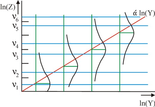
Thus the values of ε are spread according to the normal probability density-function fμ,σ(ε), also expressed as N(μ, σ²) 8. In the probit model it is assumed, that the average expected value equals E[ε] = μ = 0. The variance of the distributions is expressed by σ² = 1. This is allowed, because the scale is invariant for a linear transformation. This completely determines the model equation in the formula 1. The formula 1 is called the link function, because she couples a continuous function to discrete values.
The figure 2 shows as a schematic image the model values, that are predicted for the latent variable ln(Z). Note, that the intervals between the boundary values {νn} (the blue horizontal lines) have a variable length. The four green vertical lines represent some possible values of ln(Y), with the corresponding normal spread in the personal attitude.
Now the task is to choose such values for α and the set {νn}, that the resemblance between U and ln(Z) is maximal. For this purpose the probit method commonly uses the maximum likelihood method9. Here the criterion for the best possible fit is, that the theoretical probability for measuring the empirical collection {Uk} is maximal.
The procedure is as follows. Suppose that the individual with number k has chosen Uk=n. Then the model equation in the formula 1 requires, that ln(Z) lies in the interval <νn; νn+1]. The latent variable of the individual has the value ln(Z) = α × ln(Yk) + εk. Therefore the value of the deviation εk must lie in the interval <νn − α × ln(Yk); νn+1 − α × ln(Yk)].
Since εk has a normal distribution, the corresponding probability Prk(α, νn, νn+1) can be computed from the cumulative distribution function Φμ,σ 10. To be precise, the probability equals Φ0,1(νn+1 − α × ln(Yk)) − Φ0,1(νn − α × ln(Yk)). The reader, who is familiar with the statistical theory, will recognize this approach. The term equals the surface of the probability density-function f0,1 between the points εk = νn − α × ln(Yk) and εk = νn+1 − α × ln(Yk).
Next the maximal probability function L(α, {νn}) can be defined. Suppose that the total number of measurements in the figure 1 equals K, then the function equals L(α, {νn}) = Pr1(α, {νn}) × Pr2(α, {νn}) × ... × PrK(α, {νn}). The maximal probability estimator of L(α, {νn}) is the combination of values α, ν1, ν2, ν3, ν4, ν5 and ν6, which maximizes L. The estimator can be found by a varying those seven values over their allowed range, and computing the corresponding value of L for each combination of values. These are indeed computations, which can require an enormous effort.
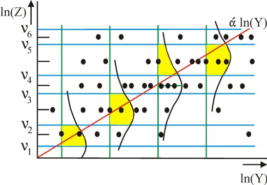
As an illustration of the presented probit method the figure 2 shows how the figures 1 and 2 can be telescoped. Moreover the figure 3 selects four measured points by connecting them with the green vertical line. According to the theory the choice for the utility value U=n requires, that ε lies between the boundaries, which correspond to n. For each measured point the surface of the probability density-function between the two boundaries is coloured in yellow. According as the surface is larger, the corresponding measured value has a larger probability of occurring. For instance, one sees that the third measured point lies in the tail of the density-function.
In this way the primary principles of the scaling and measurement of the utility (satisfaction) of the income by means of the probit method have been sketched. Van Praag and Ferrer-i-Carbonell remark that the scaling is merely possible due to the application of the quantitative latent utility function ln(Z). Although the measurement itself uses a purely ordinal scale, the validation by means of the theoretical construction actually requires a cardinal utility. Therefore the probit method is characterized by an implicit cardinal utility11.
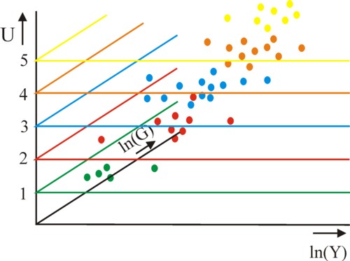
Although the length of the preceding paragraph may suggest otherwise, in fact the described case is quite simple. For many other variables can be imagined, besides the household income, which will also influence the latent utility function ln(Z). An obvious variable is the household size G. For according as the household increases, the household income must be divided among more household members. Van Praag and Ferrer-i-Carbonell have considered a large number of variables in their study, such as the number of adults in the household, the number of children, and the family structure.
When for instance the household size G is added to the formula 1, then she changes into
(2) ln(Z) = α × ln(Y) + β × ln(G) + ε
In the formula 3 an extra constant β appears, whose value must also be estimated by means of the maximum likelihood method. The figures 1, 2 and 3 become three-dimensional, because the values of ln(G) must be registered along the third axis. The figure 4 is an attempt to show the three-dimensional analogy of the figure 1, with the measured values in a different colour for each n. The points of the same colour lie in the horizontal plane of the same colour. The centre of gravity of the cloud of points shifts away from the origin.
The column ends here, because the portal dislikes extremely long ones. The reader will naturally understand, that the most interesting part is yet to come. First, Van Praag and Ferrer-i-Carbonell develop in their book also a truly cardinal scale for the utility of the monetary income. Second, they introduce an alternative indicator, which they call the income evaluation question (in short, IEQ). Here the probit method is abandoned as the means to adapt the model constants to the measured values. Instead the regression method is used, such as the linear least-squares method. These two points will be addressed in a future column.
Even more exciting than the alternative constructions is evidently the application of the methods to the really measured attitude of people. The reader can find a first result in the column about the cardinality of the marginal utility. Your columnist plans to discuss many other applications from the book of Van Praag and Ferrer-i-Carbonell on this web portal. Less interesting, but very relevant for statisticians, are the discussions with regard to the mathematical methods, which allow to calculate the error margin (confidence) of the values of the model constants. Your columnist will not address this subject - unless a reader is willing to pay for it.