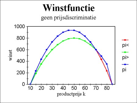
Figure 1: Profit function Π (red = duopoly,
green = monopoly, blue = envelope)
It is a paradox, that the modern theory of economics provides some support for the claim of the original social-democracy, that the industry would inevitably evolve into an ever increasing concentration. The present column discusses four models of combinations (trusts and cartels, oligopolies), copied from the book Industrial organization in context by Stephen Martin. Bundling of products is an efficient means of power. Price discrimination also has huge advantages, when the oligopoly is able to dictate these. Thanks to these techniques the combination can cleverly react to the reservation prices of the buyers. Thus a combination with a monopoly can even push her competitors and buyers from the market, if desired.
In a previous column it is stated that at the start of the twentieth century the social-democracy still believes, that the industry will inevitably become more concentrated. There a reference is made to the ideas of two leading social-democrats of the era, namely the Dutchman F.M. Wibaut and the Austrian R. Hilferding. In accordance with the then dominant paradigm they state, that it is useless and harmful to resist the progressing concentration. In many branches the trusts and cartels (also called combinations) would be necessary for the efficient production, and for preventing waste. However, the trusts and cartels have an enormous economic power, both by their capital stocks, and by their seize and monopoly position.
The consequence is that, as soon as they gain ground within some branches, they will begin to dominate the industry in the remaining, non-concentrated branches. They can dictate the cost- and sales-prices as the supplier and/or buyer in other branches. Thus the concentrated branch has the power to prescribe the profits in the other branches, so that those branches are completely at the mercy of the combinations. This can only be prevented, when indeed all branches form their own combinations. Other market forms simply do not survive. However, since some combinations will always be stronger than others, the smaller combinations will be swallowed by the large ones. The ultimate consequence of this process is that eventually a single gigantic national (or even global) combination remains1.
At the end of the mentioned column it is explained, that the scenario, sketched by the social-democracy, is not realized in practice. There are a number of reasons for this. First, the state introduces regulations, that forbid the formation of harmful combinations. Furthermore, the life span of combinations always turns out to be finite: after some time they begin to shrink. And in addition in many branches the combination is so inefficient, that it is not worth the effort to form and maintain her. But the modern theory of economic concentration can also prove, that in principle a combination has indeed the power to influence at will the other branches in her industrial column (that is to say, ancillary suppliers and buyers) by means of various manipulations. The present column elaborates on four of these models. They are copied from the book Industrial organization in context b Stephen Martin2.
On p.284 in Industrial organization in context a situation is studied where a monopoly supplies raw materials or semi-manufactured products to a duopoly (that is a branch, where merely two producers are active). Apparently the monopoly and the duopoly form (a part of) an industrial column. It is said that the monopoly is upstream in the column, and the duopoly is located downstream. The duopoly sells her product for a price p. The sales of the producer ν is qν (with ν=1 or 2). It is assumed that the inverse demand function of the duopoly product is linear, namely
(1) p = pmax − β × (q1 + q2)
The duopoly pays a price k per unit of received product to the monopoly. Furthermore, the costs in the duopoly differ, for the producer ν (with ν=1 or 2) has extra costs mν. Thus the total costs for the producer ν equal Cν = (mν + k) × qν. The marginal costs are cν = ∂Cν/∂qν = mν + k. Suppose that the duopoly is of the Cournot type, where both producers accept each other's sales as a given fact. In a previous column it is shown, that then an equilibrated market is only possible, when the sales satisfy
(2) qν = (pmax + mμ − 2×mν − k) / (3×β)
In the formula 2 μ denotes the other producer. In other words, when one has ν=1 then μ=2, and vice versa. The formula 2 shows, that the price setting of the upstream monopoly has consequences. For, when one has k ≥ pmax + mμ − 2×mν, then the downstream producer ν is eliminated from the market. Suppose that the producer 2 has the highest costs (m2 > m1), so that he is the first to leave the market. Then the producer 1 would change into a monopoly, which maximizes her profit at q1 = (pmax − m1 − k) / (2×β) 3. So two market configurations are conceivable, depending on k. For the used assumption, that each unit of product of the upstream monopoly corresponds to a unit of product of the duopoly, the sales of this monopoly equal
(3a) Q = q1 + q2 = (2× (pmax − k) − (m1 + m2)) / (3×β) for k < pmax + m2 − 2×m1
(3b) Q = q1 = (pmax − k − m1) / (2×β) for k ≥ pmax + m2 − 2×m1
Suppose that the upstream monopoly has marginal costs with a size of γ. Then her profit equals Π = (k − γ) × Q. This profit function is presented graphically in the figure 1, in the form Π = Π(k) 4. The maximization of her profit requires, that one has ∂Π/∂Q = 0. In the present situation this requirement equals ∂Π/∂k = 0. This optimum can be calculated from the set 3a-b. As long as m2 is not much larger than m1, the optimum of the upstream monopoly is located at5
(4a) k = ½×(pmax + γ) − ¼×(m1 + m2)
(4b) Π = (pmax − γ − ½×(m1 + m2))² / (6×β)
Apparently the upstream monopoly has an interest in maintaining the duopoly. In addition this example shows, that she could eliminate the producer ν=2, if desired. However, the monopoly can improve her situation even more than in this example by discriminating in her price setting. That is to say, suppose that the monopoly can demand different prices k1 and k2 from the producers in the duopoly. This will obviously only succeed, when she disposes of sufficient power to prevent, that the buyer with the lowest kν sells the goods to his competitor. Now the formula 2 is replaced by a more complex one:
(5) qν = (pmax + mμ + kμ − 2×(mν + kν)) / (3×β)
In the formula 5 ν again differs from μ. The set 3a-b will evidently change accordingly. Moreover, now the maximization dΠ=0 of the upstream monopoly leads to (∂Π/∂k1) × dk1 + (∂Π/∂k2) × dk2 = 0. Due to the independency of k1 and k2 two conditions must be satisfied, namely ∂Π/∂k1=0 and ∂Π/∂k2=0. After a lot of arithmetic the obtained result is6
(6a) kν = ½×(pmax + γ − mν)
(6b) Π = ((pmax − γ) × (pmax − γ − (m1 + m2)) + m1² + m2² − m1×m2) / (6×β)
It is striking that the end users (consumers) do not notice anything of the manipulations by the upstream monopoly. For, both without and with price discrimination one has
(7) Q = (pmax − γ − ½×(m1 + m2)) / (3×β)
Due to the inverse demand function 1 the price p is also independent of the price discrimination. So the price discrimination does not hurt the consumer market. However, it turns out that the profit Π with price discrimination becomes higher than without price discrimination. Namely, the difference between the two profits is7
(8) ΔΠ = (m2 − m1)² / (8×β)
Since the total yield on the market of end users is fixed (namely p×Q), apparently the upstream monopoly appropriates a part of the profit of the duopoly! The question rises how each of the producers in the downstream duopoly is affected by this. The formulas 4a and 6a show, that one has Δkν = kν − k = ¼×(m1 + m2 − 2×mν). Since one has ν=1 or 2, it follows that Δk1 = -Δk2. Suppose for the sake of convenience, that m1<m2. Then apparently in the case of price discrimination the upstream monopoly benefits from raising her product price k1 for producer 1, as well as lowering the price k2 for producer 2. Then producer 1 has higher costs, and therefore he will product less products. The reverse is true for producer 2. Indeed the formulas 2 and 5 show, that the formula Δqν = (Δkμ − 2×Δkν) / (3×β) = -Δkν / β is valid8.
On p.367 in Industrial organization in context the situation of the previous paragraph is studied in detail. Suppose that the upstream monopoly offers producer 1 to obtain the monopoly on the downstream market. Then the producer 1 wil try to maximize his profit as a monopoly. It is shown in the formula 3b, that this leads to q1 = (pmax − m1 − k1) / (2×β). In a footnote it is shown that then the upstream monopoly can maximize her profit by setting k1 = ½×(pmax + γ − m1). This choice still gives some profit to the producer 1 9.
However, now Martin assumes, that the upstream monopoly is guided by envy, so that she will not give up any profit to the downstream monopoly of producer 1. That is to say, the producer 1 must sell to the end users with a product price, that merely covers the costs. In that case one has k1 = p − m1. In this contract it is not allowed to the producer 1 to exploit his position as a monopoly. In fact the upstream monopoly reduces the producer 1 to a powerless link and a mere distributor. However, although the producer 1 does not make a profit, he has at least secured his existence. The contract benefits the end users, because they obtain the goods of producer 1 at a competitive price. The quantitative sales q1 is twice as large, in comparison with the situation, where producer 1 would exploit his power as a monopoly.
Note that the upstream monopoly does continue to maximize her profit, so that one must have k1 = ½×(pmax + γ − m1). So the contract imposes on the producer 1 the cost price k1, as well as the obligation to purchase q1 = (pmax − p) / β = (pmax − m1 − k1) / β = ½×(pmax − m1 − γ) / β, and (after some working) to deliver this quantity to the end users. That looks like a convenient agreement. However, the producer 1 must take into account, that the upstream monopoly will betray him (by means of a hold up), and yet supply her goods to the producer 2, at a lower price k2. For, at the given quantity q1 the inverse demand function becomes p = ½×(pmax + m1 + γ) − β×q2. So when producer 2 can supply the end users at a product price below m1 + k1, he creates enough market space to sell q2.
The upstream monopoly can help the producer 2, by offering the goods at a price k2 < m1 + k1 − m2. This second contract obviously hurts producer 1, because he can no longer sell his goods at the price m1 + k1. He must lower his price to m2 + k2, in order to compete with the producer 2, and therefore will incur a loss. Therefore producer 1 will only sign the contract with the upstream monopoly, as long as she promises not to flood the market with her goods (dumping). The most secure form of mutual obligation is the vertical integration, where the upstream monopoly simply takes over the producer 1. Thus the reader sees, that combinations indeed tend to expand into other branches, such as Wibaut and Hilferding already feared.
On p.254 in Industrial organization in context Martin describes a case of product bundling. Bundling occurs more often than one would assume at first sight. Everybody knows the case of the computer operating system, that is sold in combination with a search engine. But suppliers of cable television sell the broadcasting in packages as well. And the public regional transport bundles the transport between the cities with the transport within the cities. The American robber barons at the start of the twentieth century bundled the production of oil with its transport. Thus Wibaut writes: "In this manner the intrigues with railway tariffs have brought the Standard Oiltrust to its immense power and expansion. They implied among others, that the competitors of the trust not merely paid a much higher price for the transport of their oil than the trust, but also that this surplus was acquired by the trust itself"10.
Yet there is a certain risk in the bundled sales, at least at the start, because the bundle is actually a new product on the market. The markets of the separate products in the bundle are coupled to each other, and the effect of this is not in advance clear. Therefore the suppliers of the bundle will have to do careful market studies. Martin gives the example of a producer 1, that manufactures two products A en B. This is called a horizontal integration of the markets for the products A and B. The producer 1 has a monopoly for the product A. However, on the market of the product B there is a producer 2, that competes with him.
The producer A clearly benefits from selling A and B as a bundle. For, all consumers that buy the bundle in order to obtain the product A, automatically obtain a product B as well. That product B can no longer be sold on the market for B, where the producer 2 is active. Nevertheless, the producer 1 will first have to analyze the market demand, when he wants to increase his market power by henceforth exclusively selling the products A and B as a bundle. Martin assumes that the utility function of the consumers is given by11
(9) U(QA, QB) = m + α×QA − ½×β×QA² + δ×QB − ½×ε×QB²
In the formula 9 QA and QB are the quantities of respectively the products A and B. The parameters α, β, δ, and ε are positive constants. The term m represents the utility of various other goods, that are not relevant here. Note that the marginal utility ∂U/∂Qk (with k=A or B) decreases. Suppose furthermore, that the product prices are represented by pk. The consumers dispose of a total sum Y, which they spend entirely. A part m of it is spent on other goods than A and B. In other words, the budget restriction is Y − m = pA×QA + pB×QB. Then according to the second law of Gossen one has pk = λ × ∂U/∂Qk. For the sake of convenience choose the monetary unit such that one has λ=1. Thus the inverse demand functions on the markets of A and B without bundling are given by
(10a) pA = α − β×QA = α − β×q1,A
(10b) pB = δ − ε×QB = δ − ε×(q1,B + q2,B)
In the set 10a-b q1,A is the quantity A, that the producer 1 can sell. And q1,B and q2,B are the quantities B, that respectively the producers 1 and 2 can sell. Suppose furthermore, that the marginal costs for the producers 1 and 2 are respectively c1,A, c1,B and c2,B. In the market for A the producer 1 makes an optimal monopoly profit of π1,A = (pA − c1,A)×q1,A = ¼×(α − c1,A)² / β = β×q1,A². In the market for B there is a Cournot duopoly, and then one has in the equilibrium that qν,B = (δ + cμ,B − 2×cν,B) / (3×ε), witht ν <> μ (compare the formula 2). After insertion in the formula 1b the price is calculated as pB = (δ + c1,B + c2,B)/3. It follows that the profits in the market of B are πν,B = ε×qν,B². This implies tha the total profit of the producer 1 on both markets is πA = β×q1,A² + ε×q1,B².
Now suppose, that in future the producer will sell a product A exclusively in combination with a product B. Moreover, he no longer sells the product B separately, so that one must have q1,A=q1,B. This is precisely the quantity of supplied bundles, which henceforth will be represented by σ1. In the remainder the sales of A and B are given by QA = σ1 and QB = σ1 + q2,B. Insert these expressions in the formula 9. Then the second law of Gossen can again be applied, where however the marginal utilities must be calculated with regard to the quantities σ1 and q2,B. That results in the inverse demand functions
(11a) pσ = α + δ − (β+ε) ×σ1 − ε×q2,B
(11b) p2,B = δ − ε×(σ1 + q2,B)
The bundle and the separate product B ought to have their own demand functions, were it not that they are substitution goods. Therefore there are cross terms in the set 11a-b. The quantity σ is a given for the producer 2, whereas the quantity q2,B is a given for the producer 1. The producers 1 and 2 act on their own markets as if they are monopolies, and thus both try to maximize their profits. That leads to the best reaction functions for each of the producers:
(12a) σ1 = (α + δ − ε×q2,B − c1,A − c2,A) / (2×(β + ε))
(12b) q2,B = (δ − ε×σ1 − c2,B) / (2×ε)
The set 12a-b can be solved for σ1 and q2,B. This solution [σ1, q2,B] is the only state of equilibrium on the markets. After some cumbersome and persistent calculations one finds
(13a) σ1 = (2×α + δ+ c2,B − 2×(c1,A + c2,A)) / (4×β + 3×ε)
(13b) q2,B = (δ×(2×β + ε) − 2×c2,B×(β + ε) − ε×(α − c1,A − c1,B)) / (ε×(4×β + 3×ε))
The profit of producer 1 is π1 = (β+ε) × σ1², and the profit of producer 2 is π2 = ε × q2,B². Now the intriguing question is obviously whether the producer 1 has indeed increased his profit thanks to the bundling. Here your columnist forgoes a general answer, and following Martin considers the concrete case α=δ=100, β=ε=1, and c1,A = c2,A = c2,B = 10. According to the formulas directly below the set 10a-b without bundling one has π1 = 45² + 30² = 2925 and π2 = 30² = 900. The situation with bundling leads to π1 = 2× (270/7)² = 2975.5 and π2 = (180/7)² = 661.2. The bundling has indeed given producer 1 an extra profit, whereas the producer 2 has handed in profit.
But this does not finish the story. Namely, suppose that the producer 2 has incurred fixed costs for his production, which he pays from his profit. When his fixed costs are higher than 661.2 (and lower than 900), then due to the bundling he endures losses on his activities. He will have to leave the market, which results in q2,B=0. The formula 12b shows that then sigma;1 = 45, and therefore the profit of producer 1 equals π1=4050. Apparently there are huge advantages in pushing the producer 2 from the market12.
On p.278 in Industrial organization in context Martin describes a case, where a monopoly benefits from the product bundling. The monopoly produces two products A and B, with product prices pA and pB. Suppose that an average consumer n (with 0<n≤N) is willing to pay at most ρA,n for product A, and ρB,n for product B. The monopoly sells her product to all consumers with ρA,n ≥ pA, and she sells her product B to all consumers with ρB,n ≥ pB. The variables ρA,n and ρB,n are called the reservation prices of consumer n for respectively the products A and B. Suppose for the sake of convenience, that each of the reservation prices of each consumer is bounded by the maximum α. Consider the (admittedly, rather curious) situation, where each of the N consumers chooses a combination [ρA, ρB], that occurs just once, and where all combinations indeed occur.
That is to say, the pairs of reservation prices of the consumers are distributed uniformly across the price square with sides [0, α] × [0, α]. In short, all N consumers together fill the price square with surface α². A fraction pA×pB / α² of the consumers will buy nothing at all. The fraction of consumers that buy A is (α − pA)×α / α² = 1 − pA/α. In the same way a fraction 1 − pB/α buys the product B. Apparently the inverse demand function for the eager fraction is
(14) pk = α × (1 − qk / N) for k = A of B
Suppose that the production costs of the product k have a size ck. Then the optimal profit for each product equals πk = (pk − ck) × qk = ¼ × (N/α) × (α − ck)² 13.
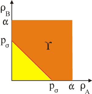
It is immediately clear, that the sales can perhaps be increased by bundling the products. For, this allows to make additional sales to each consumer, that has one reservation price far above the one product price (of A or B), whereas his other reservation price is just below the other product price (of B respectively A). The bundle price is given by pσ. Alle consumers with ρA,n + ρB,n ≥ pσ will buy the bundle. This is shown graphically in the figure 2. It is clear that no sales are made below the line, that connects [pσ, 0] and [0, pσ]. The size of the surface Y allows to derive the composite demand function as
(15a) σ = (α² − ½×pσ²) × N/α² for 0 ≤ pσ ≤ α
(15b) σ = ½ × (2×α − pσ)² × N/α² for α ≤ pσ ≤ 2× α
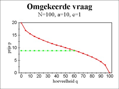
The inverse demand function of the set 15a-b is shown in the figure 3. Now the monopoly can calculate the σ, that maximizes her profit. For, the set 15a-b gives pσ as a function of σ. Then one has ∂π/∂σ = pσ − cσ + σ × (∂pσ/∂σ), and that expression equals zero in the optimum. That looks simple. Nevertheless, your columnist places the calculation of the general solution (σopt, pσopt) for the optimum in a footnote14. The main text will confine itself to just a numerical example. Following Martin concrete values are chosen for the parameters: N=100, α=10 and cA=cB=1. This implies that the costs of the bundle are cσ = cA + cB = 2. In the footnote it is shown, that a maximal profit of π = 417 is reached in (σopt, pσopt) = (60.8, 8.86).
The calculated profit can be compared with the profit, that the monopoly makes without bundling. The formula 14 has shown, that in that situation the maximal profits equal πk = 202.5 for k=A and B. Therefore the total profit equals 405. It is obtained at (qkopt, pkopt) = (45, 5.5). This shows that the bundling truly leads to a larger profit. What is the effect on the consumers of the bundling by the monopoly? Martin does not answer this question. Neither can your columnist give a useful comment. Yet here is an attempt.
It is clear, that the monopoly can sell more products A and B thanks to thier bundling, namely 60.8 of each instead of 45. Moreover, the consumers pay less for the bundle than for both separate products together, namely 8.86 for the bundle instead of 11 together. On the other hand, due to the bundling a part of the consumers are forced to buy a product, that they do not really need. These consumers are hurt by the bundling. However, their number depends on the distribution of reservation prices, and precisely these have been chosen rather arbitrarily in this model. For, the applied "uniform" distribution is not necessarily typical for all cases, where two markets are combined. This model does prove, that the market power is possessed by the monopoly, and not by the consumers. And the monopoly is merely interested in profit, and not in the welfare of the consumers15.
The present column sketches situations, where a monopoly can dictate at will product prices to her buyers. Thus she also has the power to determine her own profit, and to skim the profits of downstream enterprises. She can even ruin some of her buyers, as far as their survival depends on the supplied goods. That dependency can be an incitation for vertical integration, where a trust is formed. Horizontal integration can be beneficial for a trust as well, because after the entrance into the new market she has commonly a strong position there. The four presented examples strengthen the sombre expectations of the traditional social-democracy. But they are also a warning to politicians to be wary of model prognoses. Even when the theory predicts catastrophies and apocalypses, the reality can nevertheless develop in a different direction.