The LTV of de Wolff for two products

First insertion on Heterodoxe Gazet Sam de Wolff:: 7 may 2012

A preceding column describes the labour theory of value (abbreviated LTV) of Sam de Wolff. With her de Wolff tries to advance and innovate the traditional LTV of Karl Marx. In the labour theory of value the (exchange) value of a product is equal to the amount of labour time, that is spent on the product. The work of De Wolff is characterized by a combination of the LTV and the marginal analysis, in the way it was presented for the first time by the economist Hermann H. Gossen, and later was perfected by the economists William S. Jevons and Léon Walras. Contrary to other economists De Wolff uses the LTV mainly in order to determine the total size of the production in the society. For him the exchange value (the price) of products is of secondary importance. It is typical for De Wolff that he invents his own terminology for all the relevant quantities in his model. Thus he prefers to refer to utility with the word pleasure, and to marginal utility with the expression intensity of pleasure. The introductory column just mentionned about the LTV describes how De Wolff uses a simple Robinsonade in order to determine the most efficient size of production.

In the simple Robinsonade the society generates just one product, namely corn. But in his main work Het Economisch Getij De Wolff tries to model the more complex case of a society with a diverse product assortment. Also here the new insights of the theory of marginal utility are profitable. The present column aims to describe this extended model of De Wolff in a clear way. It should immediately be added, that De Wolff sometimes lapses into digressions, that make a strange impression on the modern economist¹. Your columnist can not judge whether De Wolff himself is confused. It may be, that the knowledge of the time just did not allow for a more clear wording.

De Wolff explains his extended model by means of an example, and this column follows in his footsteps. At the end it will be established, that unfortunately a more general formulation of the model has its limitations. In the example the one-person society disposes of two products, namely corn (like before) and fish. In the preceding column it is shown how the knowledge of the labour productivity allows to write the pleasure L as a function of the total expended labour time t. De Wolff chooses the following pleasure functions for the acquisition of respectively corn and fish
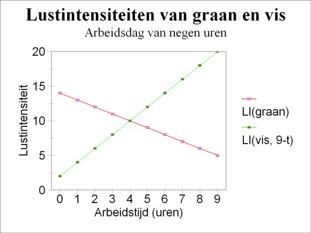
Figure 1: Example with two pleasure intensities

(1)     L_g(t) = 14×t - ½×t²

(2)     L_v(t) = 20×t - t²

The time horizon for these two pleasure functions is a labour day, and the unit of time is an hour of labour. The choice to base the pleasure on a common time variable implies, that the production value is included implicitely in the pleasure functions². Thus the pleasure in this form is distinct from the well-known utility concept, which is independent of the production price. Note that De Wolff wants to express the pleasure as formulas and therefore he is forced to apply a cardinal pleasure analysis³. The so-called pleasure intensity LI is obtained by calculating the derivative of the pleasure L:

(3)     LI_g(t) = 14 - t

(4)     LI_v(t) = 20 - 2×t

First De Wolff studies the situation, where the Robinson person has decided to work daily for nine hours. His decision fixes the displeasure O, which the person is willing to endure daily as a consequence of his labour⁴. The only thing that remains to be done is to divide his labour time as rational as possible between the harvest of corn and the fishery. The rational distribution requires, that the person optimizes his daily pleasure. Each hour of his nine-hour working day, which he spends on the harvest of corn, is lost for the fishery, and vice versa. A choice must be made from the collection of production options. Here certain profits must be given up for ever, and thus alternative costs must be made (opportunity costs). In the model the alternative costs take on the form of a lost pleasure. From the marginal analysis it is known, that the optimal combination of products is obtained, as soon as the marginal utilities of each pair of products are in the proportion of their respective prices. This is the so-called Second law of Gossen. In the model of De Wolff a transformation into labour time is carried out, by which the product value is already included in the LI. Therefore in the rational optimum the two pleasure intensities are simply equal to each other. In other words, the condition for the optimum is:
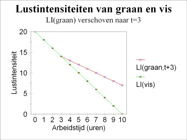
Figure 2: example with combination of pleasure intensities

(5)     LI_g(τ) = LI_v(9-τ)

In formula 5 the variable τ is the optimal quantity of labour time, which must be spent on the harvest of corn. In order to calculate τ the formulas 3 and 4 should be substituted in the formula 5. The result is τ = 4 hours of labour. In other words, the Robinson person chooses a yield of corn equal to 4 working hours and a yield of fish equal to 5 working hours. Alternatively, the formula 5 can be solved in a graphic way. The graphic approach uses the fact, that τ on the righthand side of the formula 5 appears with a minus-sign. The pleasure intensities LI_g and LI_v are drawn ih the same figure, however with the axis for LI_v extending in the opposite direction⁵. The result is shown in the figure 1. It can be read from the figure, that the intersection is indeed at τ = 4 working hours.

After this five-finger exercise De Wolff tackles the complex task of determining the combined pleasure intensity LI(t) for two products. Contrary to the situation discussed just now, here the quantity of labour time t can assume any possible value (at least, within the time horizon of the separate pleasure functions). It turns out, that the elaboration of this exercise also provides for an alternative way to solve the situation with t=9 hours. In the composition of his optimal product combination the Robinson person will check first whether one of the two products supplies a unique pleasure. An investigation of the formulas 3 and 4 shows, that this is indeed the case, for during the first three working hours LI_v(t) is always larger than LI_g(t). This is for instance clearly visible in the figure 1. Therefore these hours will certainly be spent on fishery.

From the point t=3 the situation becomes more difficult, because at that moment the harvest of corn and the fishery both supply the same pleasure intensity, the size of 14. This is shown in outline in the figure 2 by a shift of the origin t=0 of the formula 3 to t=3. Suppose that the Robinson person decides to change from fishery to the harvest of corn. As soon as he works a minute in the harvest of corn, LI_g will drop below 14, while LI_v will remain unchanged at 14. Then he is forced to engage again in fishery, at least for a moment, several seconds, until LI_v is lowered to just below LI_g. In this way he must jump back and forth between the fish and the corn. In reality this is of course impossible, so that the Robinsonade is not a very convincing choice of model⁶. Anyhow, the result of this continuous change is that the decrease of LI_g(t) and LI_v(t) with time will be the same.

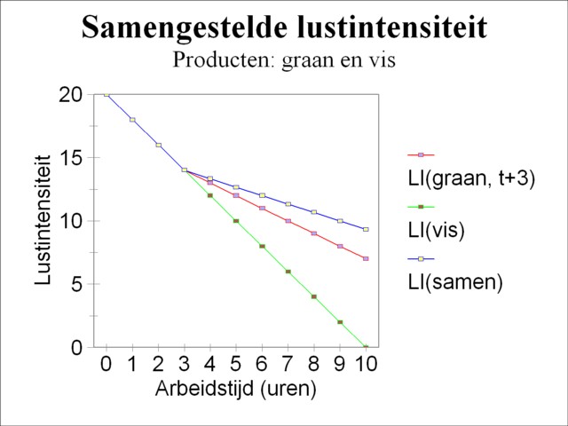
Figure 3: Example of combined pleasure intensity

Formally, the pleasure intensity from t=3 can be described as follows. At that moment one obtains LI_v(t') = 14 - 2×t' with t' = t-3 and (after the shift along the t-axis) LI_g(t') = 14 - t'. Consider the time interval Δt that follows this moment. A fraction α of this interval will be spent on fishery, and a fraction 1 − α will be spent on the harvest of corn. At the end of the interval Δt one obtains again

(6)     LI_g((1-α)×Δt) = LI_v(α×Δt).

Substitution of the expressions for LI_v and LI_g just mentionned yields the result, that the identity is satisfied with α=¹/₃. In short, a third of the time is spent on fishery, and two thirds of the time is spent on the harvest of corn. Thus the pleasure intensities of the two products and their combined pleasure intensity LI can be calculated:

(7a)     LI_g(t') = 14 - (1-α) × t' = 14 - ²/₃ × t'
(7b)     LI_v(t') = 14 - 2 × α × t' = 14 - ²/₃ × t'
(7c)     LI(t') = 14 - ²/₃ × t'

The substitution of t'= t-3 in 7c leads to LI(t) = 16 − ²/₃ × t, at least for t>3. As expected the combination of two products yields more pleasure intensity than each of the products separately. The time allocation of one third for fishery and two thirds for the harvest of corn appeals to the intuition. For according to the formulas 3 and 4 the pleasure intensity of fish diminishes twice as fast as for the corn. The labour time of fishing must as it were be slowed down with a factor of two with respect to the labour time of the harvest of corn. This is precisely what has been done by splitting each time interval into a fraction α and a fraction 1 − α.

In summary: until t=3 the combined pleasure intensity LI(t) is equal to LI_v(t), and from that moment on it is equal to the formula 7c. The figure 3 shows LI(t) in a graphical form. Until t=3 the Robinson person will exclusively fish, and after that he will spend a third of each time unit on fishery and two thirds to the harvest of corn. For t=6 there will be 4 hours of fishing and 2 hours for the harvest of corn (see also the preceding text). Etcetera. De Wolff remarks, that the order of the activities is irrelevant. In a working day of nine hours the Robinson person is free to harvest during the first 4 hours, and then to fish during 5 hours⁷.

Finally De Wolff tries to generalize his example, and he asks himself, how the pleasure intensity will vary for an arbitrary number of products. He believes that the method, which is presented in the preceding text, can be applied again for each additional product. In stead of two line segments, like in the figure 3, the pleasure intensity will exhibit a number of bends. Then the pleasure intensity gets the shape, which is presented in the figure 4. For a very large number of products she will even transform into a continuous curve. However it should be noted here, that the whole method is only applicable, as long as the pleasure of the products is of the form L(t) = c×t + d×t². Of course this form is by no means self-evident⁸. The downward inclination of the combined pleasure intensity is the equivalent of the First Law of Gossen, which in our days is also called the law of the decreasing marginal utility. The model of De Wolff clearly demands for a comparison with the conventional utility theory⁹.

1. An example is already given in the preceding column, where De Wolff introduces an unusual interpretation of the marginal utility. In the same chapter he cites from the book Grundsätze der Volkswirtschaftslehre by R. Liefman, that discusses the so-called Grenzertrag. In the present German usage this is equal to the marginal product. But according to De Wolff the Grenzertrag pf Liefman is the ratio of the marginal utility and the marginal disutility. This sort of confusion sometimes makes the text of De Wolff obscure. (back)
2. In the labour theory of value the product value w is equal to the inverse of the labour productivity ap, so w = 1/ap. Strictly speaking the labour productivity should include the amount of expended capital goods. However the model of De Wolff does not consider the capital goods. (back)
3. In a cardinal pleasure analysis the pleasure is measurable. On the other hand in an ordinal pleasure analysis it can only be ordered (put in a sequence according to pleasure size). (back)
4. It is not required that the pleasure and displeasure are in equilibrium. In other words, in this example it is not necessary to satisfy the condition for an economically optimal society, which has been defined in the preceding column, namely LI=LO. De Wolff calls such a situation rational, but not necessary economical. (back)
5. This tric is often used, for instance also in the construction of the Edgeworth Box. (back)
6. In order to be realistic, the model ought to contain at least as many workers as there are products. Then the variable t is the labour time of all workers together. The time interval can be split up through the allocation of the workers to the various productive branches. This does complicate the interpretation of the model, for the individual worker no longer searches a balance between his pleasure and displeasure. Also the individual worker no longer receives the goods, which he produces, but a proportionate share of the national product. (back)
7. De Wolff plainly states on p.445 of Het Economisch Getij: "We make the assumption (incidentally highly plausible) of the interchangeability of the successive kinds of labour". This assumption is indeed conceivable, as long as the person accurately knows his own pleasures, and in addition can perform the pleasure calculations. However, if he exclusively follows his intuitive feeling, then he wil never start with the harvest of the relatively unattractive corn. (back)
8. For instance, assume that the producty obeys the different behaviour L_y(t) = t³. Then the pleasure intensity has the form LI_y(t) = 3×t². Now it is no longer possible, like with the formulas 7a-b-c, to distribute the labour time in constant fractions in such a way, that the pleasure intensities for all products will coincide. It would depend on the time t how the labour must be allocated in ever changing proportions to the production of the various products. (back)

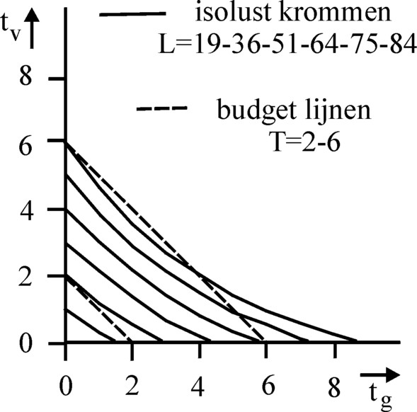
Figure 5: Iso-pleasure curves for corn and fish
9. The utility theory defines the utility as a complicated function of the quantities of products. In the example of this column the utility u could be written as u(X_g, X_v), where X_g and X_v are respectively the number of sacks of corn and the number of barrels of fish. It is usually assumed, that the iso-utility curves (that are the curves with a constant utility value) in the (X_g, X_v) plane exhibit a convex behaviour. Firstly this means that the need of the consumer for a particular product is never satiated. Secondly the consumer will never part completely with a certain product. In the Robinsonade of De Wolff a transformation to labour time is established. According to the formulas 1 and 2 the combined pleasure is L(t_g, t_v) = 14×t_g − ½×t_g² + 20×t_v − t_v². Thanks to this expression the iso-pleasure curves can be calculated in the (t_g, t_v) plane, in other words, the curves where the combined pleasure is constant. The figure 5 shows the result of this exercise. The figure demonstrates that the pleasure of the consumer does not obey the two criteria of convexity just mentionned, like in the utility theory. In the utility theory optimal product combinations can be found for a consumer with a given budget, by searching for the iso-utility curve, which is just tangent to the budget line. This iso-utility curve represents the largest utility, which can be secured by the consumer with this budget. In the same manner the optimal product combination can be found for the iso-pleasure curves. In this case the budget line is fixed by the amount of labour time T, that the Robinson person is willing to spend. In other words, the budget line is t_v = T − t_g. The method is illustrated in the figure 5 for two budget lines, with respectively T=2 working hours and T=6 working hours. This graphical presentation demonstrates why for T-values below 3 working hours the consumer only wants to acquire fish. In this area there is no point of tangency between the iso-pleasure curve and the budget line. In this case the optimal value is found on the vertical axis, at t_g=0 working hours. From T=3 working hours onwards, the budget line does touch the iso-pleasure curve. Then the consumer also wants to acquire corn. For the sake of completeness it should be noted, that from t_g=14 working hours onwards the pleasure of corn will diminish. The same occurs for the fish from t_v=10 working hours onwards. The theory of the utility of consumption can be found for instance in Micro-economie (1996, Stenfert Kroese), by F.J. Dietz, W.J.M. Heijman, and E.P. Kroese, or any other decent introduction of economics. (back)