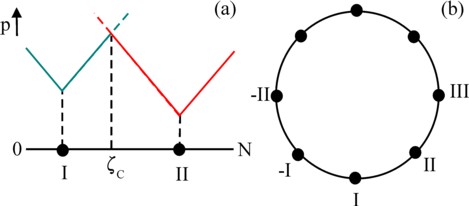
Figure 1: linear duopoly (a) and circular market (b)
It is often assumed, that markets are ruled by perfect competition. However, in practice the monopolistic competition and the oligopoly are much more common. The present column describes the possibilities for the entrepreneurs in monopolistic competition to differentiate their products. This type of market is the polypoly. The requirement of a maximal profit allows to derive the best-reaction function. The various variants of the oligopoly are also studied, namely the types of Cournot, von Stackelberg and Bertrand. The entrepreneurs can control the price or the quantity, and choose the behaviour of a satellite or initiator.
In perfect competition the consumptive demand is satisfied by the many suppliers of the same product. The market price is formed automatically thanks to the equilibrium of demand and supply. Since each supplier satisfies merely a marginal part of the demand, none of them can influence the total supply. Such a market is sketched in the previous column about price formation. Although this type of market is often presented in theoretical discussions, especially in introductory textbooks, it is not very realistic. The idea of the perfect competition is a crude abstraction. For, the offered products are never completely equal, so that various partial markets emerge. And in those practical situations where the fiction of equality is indeed approximated, a cut-throat competition emerges, which does not allow for a durable productive activity. The entrepreneurs can neither make profits, nor invest.
In reality markets are almost always of the type oligopoly or monopolistic competition. In both types the entrepreneur takes care, that he acquires an appreciable part of the total market. In the oligopoly several suppliers succeed in expanding on the market to such an extent, that they can dispose of advantages of scale. Thanks to their size they can produce more efficiently than their smaller competitors. This hinders the entrance of newcomers on the market. The expansion can be realized by forming a cartel, that is to say, an association of entrepreneurs within the branch. Sometimes even a trust is formed, where the enterprises become the daughters of the mother company. In the monopolistic competition the entrepreneurs parcel out the market by differentiating their products. This facilitates meeting the individual needs of the consumers, but it also reduces the scale of production and thus raises the prices.
During the second half of the nineteenth century the economists believed, that the oligopoly would become the natural form of the market, because she can produce so cheaply. Especially Karl Marx has made this idea popular, even to such an extent, that his successors expected the rise of oligopolies in literally all branches. This would imply, that the perfect competition is actually abnormal, and that the economy moves in a natural manner towards an organizational order. Since the twenties of the last century the idea becomes popular, that the state must accelerate the formation of this order. This political movement is described in the column about the branch corporations. In the Leninist planned economy the regime has accepted the ultimate consequence, and socialized all branches, including the agriculture, although she is totally unsuited for this. This has caused much misery, both for the producers and the consumers1.
.Reversely, in those years the monopolistic competition has been criticized much. For, it seems strange to make the products unnecessarily expensive in the then situation, where due to the universal poverty even the most elementary needs had to remain unsatisfied. The high price is caused by the small-scale production, and by the costs for advertising, which is needed in order to differentiate the product2. The supposed backwardness of the monopolistic competition has been an important argument for advancing the socialization of the concerned branches. This is a dogmatic view, which ignores the true reason for the existence of the product differentiation. For, the consumption is an important manner for people to express their identity. Thanks to the choice for a certain supplier they can shape their own style of living, and they can distinguish themselves from other people.
This column wants to reflect on the theoretical ideas, precisely because these misconceptions about the oligopoly and the monopolistic competition are so wide-spread. It is true that the various models are nor very realistic, but they do illustrate the dilemma's, which confront the entrepreneurs in such markets. The book Industrial organization in context by Stephen Martin is consulted extensively. His knowledge is supplemented with arguments from the book Grundzüge der Volkswirtschaftslehre by the authoritative German economist Peter Bofinger. In addition several other books have been consulted3.
Before discussing the theory of the oligopoly and the monopolistic competition, your columnist wants to philosophize briefly about the effect of the product differentiation on the satisfaction of consumers. Here a referral is made to a previous column about the use value of a product. In that model each product is marked by its K characteristic properties. Each property k of the product (with k=1, ..., K) takes on a value ζk. Those values can be measured in an objective way, and thus are identical for each consumer. Now consider a standard product, and for the sake of convenience define the hallmarks of this product by ζk = 0 for all k. When another product is marked by the characteristic features ξk, then the ξk are in fact the deviations with regard to the standard product. Each ξk is a differentiation with respect to the standard.
For the sake of convenience the rest of the discussion merely considers one characteristic feature ξ. Suppose that an individual consumer i attaches a utility u0 to the standard product, and that the utility decreases, according as the product deviates more from the standard. In other words, a product with the characteristic feature ξ>0 has to him a utility u(i, ξ) = u0(i) − α(i) × ξ. The constant α(i) is characteristic for the consumer i, and for the sake of convenience is taken positive here4. Furthermore, suppose that p0 is the price of the standard product. When the consumer i must buy the differentiated product for the same price p0, then he receives less satisfaction for each spent unit of money than the standard would bring him. The purchase of the differentiated product limits the real purchasing power (in terms of utility) of the consumer i. In other words, it seems as though the differentiated product has a higher price than the standard product. This increased price can be modelled mathematically as p(i, ξ) = p0 + (u0(i) − u(i, ξ)) × β(i) / α(i). The parameter β(i) is also assumed to be positive.
The preceding discussion now allows to calculate the effect of the product differentiation on the price, as is experiened by the consumer i. For, one has ∂p/∂u = -β(i) /α(i). Furthermore one has ∂u/∂ξ = -α(i). Therefore one has ∂p/∂ξ = (∂p/∂u) × (∂u/∂ξ) = β(i). Then the integration over ξ yields as the final result p(i, ξ) = p0 + β(i) × ξ. The price p(i, ξ) is subjective. In the remainder of this column it will be assumed, that β has the same value for all consumers. Then α is the only source of individuality in the model5. It must be admitted, that this argument is very abstract. However, this type of abstractions is inevitable, when an attempt is made to model the behaviour on the markets. And something is better than nothing. It allows to order one's thoughts.
This paragraph studies the product differentiation in monopolistic competition. The differentiation is represtented by the single variable ζ. Suppose that the possible values of ζ consist of the whole numbers, in the domain between 0 and N. Suppose for the sake of convenience, that there are N consumers on the market, and that each consumer has a unique preference ζ. The consumers are distributed in a uniform manner, as it where, over the domain of ζ. Thus each consumer corresponds to his own product variety. That is to say, there is a unique relation between the value of ζ and the number i, which marks the consumer. Then it seems logical to number the consumers in such a manner, that one has i=ζ. Although this is obviously an exceptional situation, she is very suited for the analysis of the market behaviour of the entrepreneurs.
Two cases will be considered: a linear scale of ζ, and a circular scale of ζ. See the figure 1. First consider the linear model: here the starting point is a market with two entrepreneurs, namely I and II. This is called a duopoly (of the Greek term dyopoly). Each of the two entrepreneurs wants to offer a unique product, so that two standard products enter the market, with characteristic features ζI and ζII. Each area of sales will increase, according as the entrepreneur lowers his product price pν (ν = I or II).
When a consumer has the product preference ζ, then his product price of entrepreneur ν equals pν(ζ) = p0,ν + β × |ζ − ζν|. The vertical bars | mark the absolute value, because here the ζ preference of the consumer can be both smaller and larger than the ζν of the standard type ν. Each deviation ζ − ζν is unpleasant for the concerned consumer6. First consider the simple case with p0,I = p0,II. Now it is clear, that each entrepreneur can best choose the middle of the range [0, N]. For, at ζI,II = N/2 the price for any consumer will not be higher than p0,I,II + β×N/2. This is called the principle of the minimal differentiation: the entrepreneurs tend to imitate each other's product.
Next consider the situation, where the entrepreneurs have chosen their own product standard ζν, which however are mutually different (ζI <> ζII). Suppose for the sake of convenience that one has ζI < ζII. Apparently the difference between the two standard products is ζII − ζI. Now each entrepreneur can only expand his sales area by lowering his price p0,ν. First consider the situation of the entrepreneur I. When he would choose p0,I > p0,II + β × (ζII − ζI), then he would evidently sell nothing. And when I chooses p0,I < p0,II − β × (ζII − ζI), then he will push the entrepreneur from the market completely. However, such a low price hurts the profit. Therefore the most interesting situation is, when I sets his price between the mentioned extremes. In that case both I and II will sell and battle to shift their mutual boundary of competition. The price behaviour is shown in the figure 1a.
A consumer with preference ζ between ζI and ζII will compare both prices. The consumer with pI(ζ) = pII(ζ) is located precisely on the competition boundary ζC. There one has p0,I + β × (ζ − ζI) = p0,II + β × (ζII − ζ). It follows that ζ = ζC = ½ × (ζI + ζII + (p0,II − p0,I) / β). Thus the sales area of entrepreneur I consists of all consumers with ζ between 0 and ζC. Entrepreneur II is preferred by the consumers with ζ between ζC and N. Due to the unique relation between ζ and the consumer number i ζC and N − ζC are the respective sales numbers qI and qII.
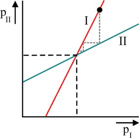
Entrepreneur I will choose the price p0,I, that maximizes his profit. Suppose that for each entrepreneur ν his variable production costs per unit are given by the constant cν. Usually cν is called the marginal costs. Then the profit of entrepreneur I equals πI = (p0,I − cI) × qI = (p0,I − cI) × ζC. The maximization requires ∂πI / ∂p0,I = 0. The result is p0,I = ½ × (cI + p0,II + β × (ζI + ζII)). This expression for p0,I is called the best-reaction function of I. She varies in a linear manner with p0,II. Note that this can be written more succinctly as cI + 2 × β × ζC. And the corresponding profit will be πI = ½ × p0,I² / β. In the same manner the best-reaction function of II can be calculated, albeit now with πII = (p0,II − cII) × (N − ζC). The result is p0,II = ½ × (cII + p0,I + β × (2×N − ζI − ζII)). She varies in a linear manner with p0,I. If desired she can be rewritten as cII + 2 × β × (N − ζC). The corresponding profit is πII = ½ × p0,II² / β.
The best-reaction functions of both entrepreneurs are shown in the figure 2. There is just one combination of p0,I and p0,II, that satisfies both best-reaction functions. That point corresponds to the market equilibrium. All other points in the plane are unstable. In principle both entrepreneurs will move towards the equilibrium. Suppose for instance, that the entrepreneur II enters the market at a later stage than I. At that moment I uses the monopoly price p0,I. Now the entrepreneur II chooses his p0,II by means of his best-reaction function. Next I will react to this move by means of his best-reaction function. Etcetera. The figure 2 shows that the prices move in steps towards the equilibrium. However, this movement is not inevitable. A stubborn entrepreneur can keep his price constant, if desired, although this will hurt his profit.
The equilibrium prices can be calculated simply by inserting one best-reaction function into the other. The result is p0,I = (2×cI + cII + β × (2×N + ζI + ζII)) / 3 and p0,II = (2×cII + cI + β × (4×N − ζI − ζII)) / 3. It is striking that these equilibrium prices increase, according as each entrepreneur moves in the direction of ζ = N/2. And it has just been proven, that rising prices drive up the profits πν. It seems as though the best position for both entrepreneurs is the middle. On a closer inspection this is a misconception, because the situation πν blocks this option. In the middle both entrepreneurs would engage in a price war, so that one of them would completely lose his sales area. In other words, the situation of equilibrium comes into existence only, when each of the two entrepreneurs differentiates his product sufficiently.
As the second case of monopolistic competition this paragraph presents the circular model. In this case the scale of the characteristic feature ζ is represented by a circle, such as is shown in the figure 1b. This circular world is formed from the linear model, when there both ends are coupled together. Thanks to this mathematical trick the circular market can be constructed with many entrepreneurs. This is called a polypoly. The circular world guarantees that all entrepreneurs have two neighbours. Strictly speaking the trick is a somewhat surrealistic operation, which remembers of the stairs of the designer Esscher7. In the figure 1b there are eight entrepreneurs. When the analysis is restricted to a single entrepreneur from this group, then it may be hoped that the specific character of the circular world has little effect on the findings.
Suppose that each entrepreneur differentiates his product with a constant difference Δζ with respect to his two nearest competitors, as is shown in the figure 1b. When the circumference of the circle is N, and there are M entrepreneurs, then one has Δζ = N/M. Furthermore suppose, that each pair of neighbouring entrepreneurs grants each other half of the in-between market segment Δζ. Suppose for a moment, that all entrepreneurs secretly decide to set the same price p0. Let pmax be the maximum price, that the consumers are willing to pay for a type in the product group. The entrepreneurs can not exceed that price (p0 < pmax).
Now the entrepreneur I wants to investigate whether he can increase his profit by choosing p0,I in a convenient manner. So he decides to withdraw from the cartel. As long as I takes care that p0,I is larger than the cartel price p0, he does not conflict with the cartel. He remains a monopolist on his market segment. His market is limited by ζmax, which is calculated from pmax = p0,I + β × |ζmax − ζI|. In other words, the sales market is |ζmax − ζI| = (pmax − p0,I) / β. Apparently in this case the entrepreneur I gives up a part of his market to the two nearest entrepreneurs. Since there is a unique relation between ζ and consumer n, the entrepreneur I can sell on both sides of his location a total quantity qI = 2 × |ζmax − ζI|. So qI = 2 × (pmax − p0,I) / β. The profit is πI = (p0,I − cI) × qI. This profit is maximal for p0,I = (cI + pmax) / 2. The corresponding sales market is limited by |ζmax − ζI| = ½ × (pmax − cI) / β.
As soon as the entrepreneur I chooses p0,I < p0, he starts to compete with his neighbours. He is no longer a monopolist. The boundary of competition at the right-hand side is pI(ζC) = pII(ζC). Completely analogous to the linear model it follows that ζC − ζI = ½ × (ζII − ζI + (p0 − p0,I) / β). In other words, the sales area on the right-hand side is limited by ζC − ζI = ½ × (N/M + (p0 − p0,I) / β). The same argument holds for the left-hand side. Thus the total sales quantity is qI = N/M + (p0 − p0,I) / β. After some reformulation the price is found: p0,I = p0 + β × (N/M − qI). Note that now the function p0,I(qI) decreases faster with qI than in the situation of a monopoly. For, there the decrease is -½×β × qI. This necessity to significantly lower the price is caused by the competition with II on the right-hand side (and -I on the left-hand side)8.
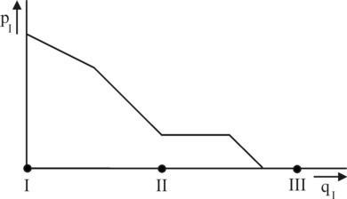
The situation with p0,I < p0 − β × Δζ is worth discussing. For, then the entrepreneur I pushes away his nearest entrepreneurs II and -I (on the left-hand side) even from their own location. Both neighbouring entrepreneurs are eliminated from the market. Therefore the entrepreneur obtains the sales markets of both II and -I. Now he enters in competition with his new neighbours, namely the entrepreneurs III on the right-hand side and -II on the left-hand side. The boundary of competition can again be calculated in the now familiar manner, but this time with a spacing of 2×N/M. The price obtains the form p0,I = p0 + β × (2×N/M − qI). The figure 3 shows the total demand curve p0,I(qI) for the three considered price ranges.
Consider again the situation in the middle price range of the figure 3. The entrepreneur I can maximize his profit by choosing the optimal value of p0,I or qI (which both give the same result)9. The optimal price is p0,I = ½ × (cI + p0 + β×N/M), which is not necessarily identical to the lower boundary of the price range. Apparently it does not always make sense to eliminate the nearest competitors. Suppose also that the marginal costs c are equal for all entrepreneurs, then the entrepreneur I is naturally not fundamentally different from the other M−1 entrepreneurs. So in the state of equilibrium the entrepreneurs will prefer the same p0,I=p0 as the rest. After insertion in the derived price formula the final result is p0 = c + β×N/M = c + β×Δζ. According as the number of enterprises M increases, the price must fall. In the limiting case of very many enterprises the price can even become equal to the production costs, just like in perfect competition.
It is difficult to model the oligopoly, because merely a few enterprises are active on the market. Therefore the developments depend strongly on the mutual interaction between the market parties. There can be a leader (also called initiator), which acts as he desires, independent of the behaviour of the others. There will certainly also be followers (also called satellites), who attune their behaviour to the actions of the other entrepreneurs10. When two entrepreneurs claim the position of leader, then a price war will result. In the oligopoly the entrepreneurs can control the market. Some models assume, that each entrepreneur ν will use his production quantity qν as a steering parameter. Other models assume, that each entrepreneur ν will steer the market with his product price pν. It is not a priori certain which model is best. That depends simply on the preferences, that the entrepreneurs will develop under the given circumstances.
Henceforth this paragraph is restricted to the case of the duopoly, where the market is dominated by merely two entrepreneurs. By definition their products are equal. An example is the market for airplanes, where Airbus and Boeing form a duopoly. Models with the quantity qν as the steering parameter are of the Cournot type. The totally supplied quantity is Q = qI + qII. The demand curve is given by p(Q) = pmax − β×Q. The entrepreneur I takes qII as a given number, and maximizes his profit by calculating the optimal quantity qI. That leads to the now familiar solution qI = ½ × (pmax − cI − β×qII) / β. This is the best-reaction function of the entrepreneur I.
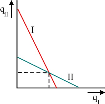
When de indices I and II are exchanged, then the best-reaction function of the entrepreneur II results. The figure 4 shows both best-reaction functions in a single coordinate system. It is clear, that only the intersection of the two lines is a state in equilibrium. In case of two satellites it can be expected, that the market stability will be realized in the end. The coordinates of the intersection can be calculated by inserting one best-reaction function into the other. The result is qI = (pmax +cII − 2×cI) / (3×β), and qII = (pmax +cI − 2×cII) / (3×β). Note that in the equilibrium the enterprise with the lowest marginal costs will acquire the largest market share. Furthermore, for the special case cI = cII = c one has Q = qI + qII = 2 × (pmax − c) / (3×β). In comparison with a market with perfect competition, where one has Q = (pmax − c) / β, the production of the oligopoly is apparently lower (namely 67%).
Next consider the discussed duopoly, where however the entrepreneur I is an initiator. The entrepreneur II continues to behave as a satellite. This is a model of the von Stackelberg type11. The entrepreneur I succeeds in discovering the best-reaction function of the entrepreneur II. Now I can insert this function in his original demand curve p(qI), resulting in p(qI) = (2×pmax + 2×cII − cI) / 3 − β×qI. The entrepreneur I uses this demand curve to maximize his profit by choosing the optimal qI. The result is qI = (pmax +cII − 2×cI) / (2×β), so 50% larger than in the case of a follower. Since the entrepreneur II is a satellite, he uses his best-reaction function and prefers qII = (pmax + 2×cI − 3×cII) / (4×β). In the special case cI = cII = c one has Q = 3 × (pmax − c) / (4×β). That is merely 75% of the production in perfect competition.
Models where the price pν is the steering parameter, are of the Bertrand type. Here the entrepreneurs are confronted with a dilemma. Namely, suppose that the entrepreneur II chooses a price pII. Then the entrepreneur will sell nothing for pI > pII, whereas reversely he will acquire the whole market for pI < pII. Obviously I will prefer the second alternative. However, the entrepreneur II will not accept this, and he will lower his price below pI. This interaction will repeat itself, until the point where one of the entrepreneurs reaches his marginal costs cν. Apparently both entrepreneurs sell their products at cost price for the case of identical costs cI=cII. At that point their profit is maximal, but unfortunately also zero. This is precisely the situation, that also occurs in markets with perfect competition.
Apparently the method of Bertrand for steering the market is not very convenient. For, a profit does become possible, when the Cournot method is chosen. But in reality both entrepreneurs will evidently decide to differentiate their two products a little. Here the reader recognizes the previous discussion about the degree of differentiation on the linear market. Now each entrepreneur has his own best-reaction function, which expresses the price that he must use as a reaction to the price of his competitor. The two lines can be drawn in the same coordinate system, just like has been done in the figure 2. In the intersection the two prices are such, that a stable market is formed. However, the differentiation reduces the advantages of the oligopoly, such as standardization and advantages of scale.
The oligopoly is indeed attractive due to her efficiency. Unfortunately this property is counteracted by the large market power, which is shared by merely a handful of entrepreneurs. The models show, that those entrepreneurs can push up their profits, and in the process will produce less than a market with perfect competition. It is understandable that politicians, especially social-democrats, advocate a supervision on the oligopolies. But on a closer inspection this solution is not satisfactory, because they substitute the entrepreneurs by politicians and civil servants. That can lead to excesses, that undermine the efficiency of the oligopoly. Therefore the best system turns out to be a mixture of entrepreneurial freedom and state supervision, where in addition some product differentiation is always present. Incidentally, as soon as the consumers dispose of sufficient spending power, the differentiation even becomes desirable.