
Figure 1: Quartet card
Catholic youth work
In a previous column the social utility of education has been analyzed. The professional literature about this theme often uses models. Several of these models are presented in the present column. It concerns two models of human capital, including a find by Mincer. The demand-supply model of Tinbergen is also explained succinctly. All of these models use econometrics in order to make them applicable for policy recommendations.
In a previous column the effect of education at the macro level of the economy has been studied. The text is mainly descriptive and narrative. During the past decades it has become more and more common to translate economic theories in mathematical models. This is useful, because in this way the causal relation between the social phenomena is presented in a succinct manner. Moreover, models enforce a clear formulation of the simplifications and assumptions. And finally, mathematical formulas allow to calculate social relations numerically, at least in principle. So there is sufficient reason to present several models of policies of education. This is accompanied by a warning: those who understand the model, do not automatically also understand reality. A model is nothing more than an abstract line of thought.
This paragraph consults the contents of the book Labor economics (in short LE)1. Nowadays the theoretical school of human capital dominates in the economic analysis of the institutional education. Taking an education is seen as a decision to invest. The potential student compares the costs O and benefits L of education. The material costs are the expenditures for the study, and the time spent on studying, which is lost for acquiring an income. But there are also immaterial costs, namely the effort of learning. The benefits of education become only apparent in the long run, namely a better job, in a challenging and autonomous function. The chance of pleasure on the job (job satisfaction) during the career increases (p.92 in LE). The humanistic theory of education also points to direct benefits, thanks to the pleasure of studying.
Suppose for the sake of convenience, that the costs O are made during the period between t=0 and t=τ. The yearly benefits are uncertain, and are only acquired during the life at work. Benefits are valued less, according as they are farther in the future. For each year of delay of certain benefits the individual devalues them with a discount factor δ. Obviously δ<1 holds, so that one can write δ = 1/(1+d), where d>0 is the individual profitability. Let T be the duration (in years) of the career. Then the utility of the investment in education equals2
(1) u = -O + Σt=τT δt × L(t)
In the formula 1 the benefits are evaluated for each year. This is a discrete process. Theoretically the benefits can also be evaluated continuously. This changes the value of the profitability, because during the whole year there is an accumulation of profits. This is to say, there are profits on profits. When r is the profitability for a continuous evaluation, then the corresponding yearly profitability equals d = er − 1 3. So one has d≥r. The continuous evaluation can be theoretically convenient, because now the sum of the formula 1 changes into an integral
(2) u = -O + ∫τT e-r×t × L(t) dt
Here (good) education increases the stock of human capital k(t). It is logical, that the capacity to learn increases, according as more k(t) has been accumulated. Then the change in human capital is given by (p.72 in LE)
(3) ∂k/∂t = κ × s(t) × k(t)
In the formula 3, κ is the intrinsic skill of the individual to learn. It is constant during his life. The function s(t) represents the fraction of the day, where the individual learns or is educated. Suppose for the sake of convenience, that the individual chooses between only working or only learning. Then s(t) is a step function, with a value of respectively 0 or 1. Because of this assumption, s(t) is eliminated from the model. It is true that s(t) is useful, when for instance part-time studies must be evaluated, or company trainings, or acquiring experience on the job (learning by doing). Suppose, that at t=ξ the individual starts an education with a duration of τ. One has s=1 for t in the interval [ξ, ξ+τ]. Thanks to the formula 3, it is easy to calculate, that therefore the individual increases his stock of human capital from k(ξ) to k(ξ) × eκ×τ.
Suppose that the wage of the worker is given by w(t) = λ × k(t), where λ is a constant (p.72 in LE). The quantity of human capital determines the productivity of the individual, and therefore his wage. Furthermore, assume that the costs O of education are determined only by the forgone wage w. The benefits L of education result from the increase in wage, namely Δw(τ) = λ × k(ξ) × (eκ×τ − 1) = w(ξ) × (eκ×τ − 1). Insert these formulas in the formula 2, then the result is (p.72 in LE)
(4) u = - ∫ξξ+τ e-r×t × w(ξ) dt + ∫ξ+τT e-r×t × Δw(τ) dt
The calculation of the integrals leads to
(5) u = (e-r×τ − 1) × w(ξ) × e-r×ξ / r + (e-r×(ξ+τ) − e-r×T) × Δw(τ) / r
The individual will choose the duration τ, which maximizes his utility. This is to say, he tries to find the solution of
(6) ∂u/∂τ = -e-r×(ξ+τ) × w(ξ) − e-r×(ξ+τ) × Δw(τ) + (e-r×(ξ+τ) − e-r×T) × (∂Δw/∂τ) / r = 0
After some simple rearrangements one finds
(7) r/κ = 1 − e-r×(T-ξ-τ)
The formula 7 implies, that r<κ must hold (p.73 in LE). Apparently education is only profitable, when the intrinsic capacity to learn is greater than the rate of return of education. And the investment in human capital will yield more profits, according as the end T of the career is farther into the future. Furthermore, the formula 7 gives the optimal duration, namely (p.73 in LE)
(8) τ(κ) = T − ξ + (1/r) × ln(1 − r/κ)
However, this result can be formulated more precisely. For, ∂u/∂τ in the formula 6 is the marginal utility of learning at the time τ. Differentiate this marginal utility with respect to ξ, then one finds4
(9) ∂(∂u/∂τ)/∂ξ = w(ξ) × eκ×τ-r×(ξ+τ) × (κ² / r) × (e-r×(T-ξ-τ) − 1).
All terms on the right-hand side of the equality are positive, except for the last one, which is negative. Apparently one has ∂(∂u/∂τ)/∂ξ < 0. The marginal utility of learning increases, according as the study is delayed more. Therefore the individual realizes his optimum by choosing ξ=0. The study must precede the career. And ξ=0 must also be inserted in the formula 8, in order to obtain the optimal duration τ.
The mentioned model illustrates well the advantages of mathematical models. The decision to study can be expressed in a few simple variables, such as κ, r, and T. Next the dependent variables ξ and τ can be derived. On the other hand, it must be admitted, that the results are rather trivial, especially ξ=0. Nevertheless, the present model can be extended further with assumptions, so that also the more complex situations can be analyzed. Consider for instance the following alternative for the formula 3 (p.75 in LE):
(10) ∂k/∂t = κ × (s(t) × k(t))α − β × k(t)
In the formula 10, s(t) can now assume all values between 0 and 1. The individual can study, in addition to his activities on the job. Then the wage is w(t) = λ × (1 − s(t)) × k(t) (p.76 in LE). The exponent α lies between 0 and 1, and therefore guarantees, that although the capacity to learn increases with k, it does so in a decreasing degree. The constant β is also between 0 and 1, and represents the devaluation of the learned knowledge. Therefore the stock of human capital decreases, unless investments are made in new knowledge.
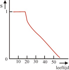
Now the individual must make a choice for the dynamics of his study behaviour s(t). He will choose s(t) in such a way, that the utility u is maximal for his career as a whole. The mathematical solution of this problem can be found with a standard technique, namely the formulation of the so-called Hamiltonian H(s(t), k(t)). The Hamiltonian replaces the well-known Lagrangian L, when the optimalization problem is dynamic (dependent on the time t). Your columnist will not bore the reader with the method to solve this optimization problem5. On p.76 and further in LE the behaviour of s(t) is presented for two cases with specific values of α, β, λ, r, k(0), T and κ. For instance: the profitability is 5%. The assumption is, that the individual starts to learn at the age of five, and that this is the time t=0. Then he already has a human capital of k(0)=5. The pension is planned at the age of 65 (5+60; T=60).
In the first case the outcome is, that the individual studies continuously (s=1) until his 23th (5+18) birthday. Then s decreases, first rapidly, and gradually more slowly. See the figure 2. The point s=½ is reached at 37 (5+32) years, and at 63 (5+58) years s=0 holds. Apparently it is possible to model the life of a college graduate by choosing suitable constants. Since the model implies the calculation of s(t), next also k(t) and w(t) can be calculated. Moreover the model succeeds in modelling the life of a person with a highschool education, by simply choosing a lower value for κ (κ=0.4 instead of 0.5) (p.78 in LE). This individual will sooner diminish his efforts to learn. The continuous education ends at 17 (5+12) years. The point s=½ is reached at 33 (5+28) years. The similarity with reality is impressive. This does obviously not means, that all of the made assumptions are sound.
The founders of the school of human capital are J. Mincer, Th. Schultz and G.S. Becker. The paragraph 2.4.1 in Labor economics discusses the models, which Mincer has proposed. They will be explained here. Suppose that the individual has a wage w(ξ) at the time ξ. Suppose that now he starts to study, and for his expenditures O only takes into account the forgone income w. Thanks to the study his wage will later rise with Δw. The individual will be indifferent for learning or working, when one has that the study yields an extra utility u=0. In this situation the formula 2 will again be applied. The profitability for u=0 is called the internal rate of return of education. However, the individual starts with the evaluation of the benefits at the time ξ, and not at the time 0. The duration τ remains undetermined for the moment. Therefore the formula 2 changes into (p.86 in LE)
(11) u = 0 = -w(ξ) + ∫ξT e-r×(t-ξ) × Δw dt
Performing the integration in the formula 11 yields
(12) Δw / w(ξ) = r / (1 − e-r×(T-ξ))
When the date T of retirement is still far away, then T is much larger than ξ. During the study one has approximately Δw / w(ξ) = r. Integrate this with respect to the duration τ, then one finds w(τ) = w(0) × er×τ. This formula represents the rise in income thanks to education. Mincer tries to explain the American incomes in the year 1959 with his formula, and finds the empirical value r=7% (p.87 in LE). However, the correlation coefficient is disappointingly low. This is actually logical, because in reality the wages continue to rise during the whole career. Therefore Mincer develops an alternative model, which takes into account the skills, which are appropriated at work. First the individual engages in a period τ of study, and then accumulates a human capital k(τ). Just like in the argument immediately after the formula 12 one finds the formula k(τ) = k(0) × er×τ.
Now let ξ be the time, which has passed since the entrance upon his duties. Assuming that the study started at the time 0, then one evidently has t=τ+ξ. During the time ξ at work the individual becomes experienced, and acquires skills. A part of the tasks has a routine character, so that merely a fraction s(ξ) contributes to the increase in human capital k. Let μ be the capacity to learn of the individual during his activities, then an analogy of the formula 3 results (p.87 in LE):
(13) ∂k(t)/∂t = μ × s(ξ) × k(t)
The formula 3 can not be solved in an exact manner. Therefore Mincer assumes, that one has s(ξ) = σ × (1 − ξ/T). Here σ is a constant between 0 and 1. Divide the left- and right-hand part of the formula 13 by k, and integrate with respect to ξ from 0 to x. The result is
(14) k(τ+x) = k(τ) × eμ×σ×(x − ½×x²/T)
The expression for the development of k(τ) can yet be inserted in the formula 12. By analogy with the model in the previous paragraph the wage at t=τ+x is calculated as w(τ+x) = λ × (1 − s(x)) × k(τ+x). The term 1-s(x) is added, because the assumption is, that the individual receives less wage because of his learning by experience. Thus finally the following formula is derived
(15) w(τ+x) = λ × (1 − s(x)) × k(0) × er×τ × eμ×σ×(x − ½×x²/T)
When desired, λ × k(0) can yet be defined as the wage w(0), which an uneducated individual would receive. Mincer has also applied this formula to the data of the American incomes in the year 1959. Then he finds the empirical values r=11% and μ×σ=8%. Since σ<1, μ>8% must hold. It turns out that the estimation with the formula 15 yields a better correlation coefficient than the formula 12 (p.87 in LE). It must be admitted, that the model of Mincer is less elegant than the model in the preceding paragraph. But it does excel in simplicity.
A previous column has already succinctly discussed the demand-supply model of Tinbergen. In this paragraph the model will be explained in detail. The book Income distribution (in short ID) has been consulted. Besides, here and there comments in the book De prijs van gelijkheid (in short PG) have been added6.
Tinbergen believes, that the spread in the attended studies is an essential cause of the inequality in incomes. Thus the state disposes with education of an instrument for making the society more equal (p.151 in ID). Notably the welfare of the various categories of workers must be equal7. Tinbergen measures this welfare with a cardinal utility function, which has already been discussed in a previous column8. The individual utility is determined by the properties tk of the individual k, and by the requirements sk of his job. In this manner Tinbergen has developed a model of the labour market. The present paragraph adapts this model somewhat in order to derive a theory of the policy of education. Then tk is the education of the individual k, and sk is the requirement of education for his position at work. Suppose that k receives a wage yk. Now the utility function of the individual is (p.60 and 62 in ID)9
(16) u(t, s) = ln(y − c0×s − c1×t − c2 × (s − t)²)

In the formula 16 c0, c1 and c2 are constants, which must be determined empirically. The formula 16 has a clear similarity with the theory of human capital. For, according as the individual k studies longer, t increases, and this must be compensated by a higher wage y 10. The model of Tinbergen uses three types of education: primary (t=1), secondary (t=2), and tertiary (t=3). The hallmark of the formula 16 is, that the job (s) of the individuals often does not coincide with their education t. This poor match leads to discontent or tension for k, which is expressed by the quadratic term. When Tinbergen designed his model, during the early seventies, the tension was still mainly due to the scarcity of college graduates. Therefore the less educated workers had to accept functions, for which they were actually insufficiently qualified.
The formula 16 can be interpreted in the sense, that it describes the utility of a representative worker with an education t. In the simplest situation this worker is indifferent between the positions s=t and s=t-1. He is prepared to accept a position above his level, because the wage always compensates entirely for the tension. For this the formula 16 can be used at a given t to derive the condition Δy = ys+1 − ys = c0 + c2 × (1 + 2×(s − t)) (p.62 in ID). The many personal properties of the worker are irrelevant. The model does order the workers in categories according to their degree of personal autonomy z (p.63). An individual has a z of 0, 1 or 2. The most autonomous characters (z=2) naturally find jobs in management or in the free professions. The autonomy does not affect the utility uk, except of course by means of the wage. It is only necessary (and indispensable!) for ordering the empirical data.
The formula 16 and the theory of human capital in principle describe the supply-side of the labour market. However, the terms with s in the formula 16 show, that the demand-side is also important. It is the uncertain demand, which makes a study somewhat risky, so that it is a speculative investment. Therefore Tinbergen develops a demand-supply model, which describes both sides of the market (p.151 in ID). There are three professional positions s=1, 2 and 3, where the value of s also refers to the required education. Tinbergen assumes, that higher educations are scarce to such an extent, that t≤s is always satisfied. Moreover there is a lower limit t≥s-1. Define nst as the fraction of the professional population, which works in the position s and has an education t. Then one must have n11 + n21 + n22 + n32 + n33 = 1. The distribution of education is given by ν1 = n11 + n21, ν2 = n22 + n32, en ν3 = n33.
Now Tinbergen describes the demand side as a production function of the Cobb-Douglas type with the form (p.82 in ID)11
(17) Y = C × (n11 + π21 × n21)ρ1 × (n22 + π32 ×n 32)ρ2 × n33ρ3 × Kρ4
Here Y is a production function at the macro level. It defines the economic structure, including the common production techniques. There are four production factors, namely workers with an education t=1, 2 and 3, as well as the factor capital K. The factor capital does not play a role in this model, because K and the power ρ4 are kept constant (p.83). The first and the second term in the formula 17 both sum the workers with t=s and t=s-1. The workers with an education t, who work in the sector s=t+1, are in a relatively high position (in comparison with their education). The factor πs,s-1 expresses, that the workers with education t and a position s=t+1 are more productive than the same workers with a position s=t. In other words, πs,s-1 > 1 holds. The higher position is labour-reinforcing, as it were.
Tinbergen assumes, that the production function is linear-homogenous, so that one has ρ1 + ρ2 + ρ3 + ρ4 = 1. It is well known, that for such a case the value ρj is the share of the production factor j in the yield Y. Therefore the formula 17 fixes the primary incomes of the three types of workers (t=1, 2 and 3). For t=1 (s=1 and 2) and 2 (s=2 and 3) they are given by (p.87)
(18a) yt,t = ρt × Y / (nt,t + πt+1,t × nt+1,t)
(18b) yt+1,t = ρt × πt+1,t × Y / (nt,t + πt+1,t × nt+1,t)
For t=3 one finds y33 = ρ3 × Y / n33. The demand- and supply-side of the labour market are in equilibrium, when one has Δyt = yt+1,t − yt,t = c0 + c2. Suppose also, that πt+1,t depends only on nt+1,t (p.86)12. Now, for a given distribution νk of education it can be calculated, how large the fractions of workers n21 and n32 are, who want a job above their level of education. This completes the model of education by Tinbergen. Levelling can be achieved by a policy of education, which lets νk approach the distributed income ρk, which is determined by the economic structure. For, this reduces the scarcity of the production factors (p.114 in ID). This will only succeed when indeed the population disposes of sufficient intrinsic capacity to learn (p.114). Tinbergen also shows, what will be the effects of a progressive income tax (p.110). Then the secondary income ηst is determined by the decision to accept a job above the level of education.
The demand-supply model of Tinbergen has the advantage, that a social welfare function W can be formulated. Tinbergen chooses the utilitarian welfare function, with equal weights for all individuals. Then it obtains the form (p.117 and further in ID)
(19) W(u) = Σt=13 Σs=t3 nst × u(t, s)
In the formula 19 one has n31 = 0 because of t≥s-1. Suppose that a tax τst is imposed, in such a manner that the secondary income equals ηst = yst − τst. Then the social optimum of W is found by varying nst, ηst and Y. Tinbergen calculates this with the empirical data of the Netherlands in 1962. The optimization of a utilitarian W usually does not lead to identical individual utilities (although Tinbergen advocates this as the just distribution). However, in the demand-supply model of Tinbergen u(s, t) is indeed equal for all groups (s, t) (p.119 and 132 in ID)13. It turns out that for the optimal W at a given t the tax τst no longer depends on s. This implies, that the tax is purely determined by the individual capacity to learn. Such a tax is called a lump sum, because within a t-group it is independent of income.

Tinbergen notes, that such an optimization of W can be done with two different assumptions. The first approach assumes, that the continued study is limited structurally by the individual capacity to learn, and therefore keeps νk constant. Then it turns out that τst becomes strongly progressive, according as t rises, with even a negative tax (this is to say, a subsidy) for the lowest group t=1 (p.120). This significantly levels the secondary incomes. Tinbergen notes, that the calculated numbers agree roughly with the reality in the Netherlands. The second approach assumes that the individuals continue to learn until s=t, and all tension is removed from the labour market. In other words, n21 = n32 = 0 holds. In this manner ηtt can be levelled even more (p.121). Obviously the level of education in the population also rises. Such a policy implies a reduction of the individual rates of return of investments in education (p.177 in PG).
Tinbergen emphasizes, that in his model the economic structure (the production function Y) does not change. In reality the technical progress creates an increasing demand for college graduates. Therefore the ρ3 in the formula 17 will become larger. The rate of return on college studies rises. Thus the policy of education and the technical progress are engaged in a race, where the effect on the social inequality is not clear in advance (p.156 in ID). Tinbergen, who is an energetic supporter of central planning, advocates to manage the technical development in such a manner, that no selective scarcity occurs on the labour market (p.156 and further in ID)! Here Tinbergen proves to be a traditional social-democrat. Nowadays this view is no longer popular. The present standard textbooks about macroeconomics all promote private markets in college education and in research14.
Furthermore, according to Tinbergen it is conceivable, that the distribution νt is determined by the innate capacity to learn of the population (p.121, 148 in ID). He assumes that perhaps a tax can be imposed in such innate talents! Even your columnist, who is yet an enthusiastic adherent of psychological research, believes that this is an unrealistic proposal. There are no reliable measurements of talent. And the distinction between innate and learned talents is diffuse. The learning of talent must not be discouraged (p.195 in PG)15. Jacobs warns on p.199 in PG, that high subsidies for universities will lead to over-investments in education and to welfare losses. Moreover they are regressive, and this actually increases the inequality (p.199 in PG). On p.200 in PG he prefers levelling by means of progressive taxes. In general the utopian desire for equality (of incomes) has disappeared from science.
In conclusion: the demand-supply model places the theory of human capital and of screening in a much wider macro-economic frame. Thanks to the production function the model can calculate the rate of return of investments in education. For, this profitability partly depends on the scarcity of college graduates. This all makes the model theoretically valuable. The ingenuity is impressive. But the model also has the ambition to be applicable to practice. It belongs to econometrics, just like the model of Mincer. This deserves a comment.
The model gives a fair description of the Dutch labour market. Nevertheless, the simplifications and assumptions in the model are rather bold, and they are sometimes difficult to reconcile with the dominant theoretical ideas. The value of such an empirical model lies mainly in the possibility to do accurate numerical predictions. Unfortunately the demand-supply model sometimes fails. On p.74 in ID Tinbergen states, that the utility function (formula 16) is applicable to the American state of Illinois, but not to Texas and South-Carolina. In these latter two states the model finds a negative value of the tension constant c2, so that the tension would lead to a positive individual utility(p.74 in ID)! Furthermore it is a bad sign, that the model has not received much scientific approval. And the model has not become common in the policy planning as an instrument for numerical calculations.