
Figure 1: Quartet card
Raiffeisenbank
Decisions can have far-reaching consequences for the future. Therefore the economic science has invented models, that allow to calculate the consequences of decisions. They attach an inter-temporal discount to the utility function. The present column extends the Walrasian model with an inter-temporal utility. Next it is applied in an overlapping generation (OLG) model. Some criticism by behavioural economics is discussed. Finally, it is explained how Van Praag discounts memories and expectations in the utility optimization.
Economic decisions are never made in a static situation. Life is dynamical. The individual and his society are subjected to continuous changes. On the one hand, each decision in the present will influence the future welfare, and on the other hand, the future decisions must perhaps be adapted to the expected developments. A familiar example of the influence of time is the valuation of future monetary incomes. Suppose that the actor k has a claim to the payment of a sum of money, which now (say, on time t=0) has a value of p0. When the payment is postponed with a time period Δt, and the interest rate in that period equals r, then k misses an income from interest with the size of r×p0. It is obvious that k wants to be compensated for his loss (discount), so that at the time t=Δt he demands a sum of money equal to p0 × (1+r).
This argument can be extended to arbitrarily long periods. For instance, suppose that the delay is tn = n×Δt, where n is a natural number. In that case, at that time a sum of money equal to p0 × (1+r)n must be paid as a compensation. For the sake of convenience, represent that sum by pn, then apparently one has1
(1) p0 = pn / (1 + r)n
In other words, when the sum pn is only paid at tn, then the present value is less than pn. The economic reason is naturally, that the sum pn can be used in a productive manner during the n periods. It is potentially an investment, which yields a profit. A second argument, that incites the actor k to demand an interest, is that during the n periods the sum is not available for his consumption. He must live in a sobre manner, and that is unpleasant. It is a burden, which must be compensated.
This latter argument can be generalized. It turns out that individuals commonly prefer a direct pleasure instead of postponing the experience of pleasure. Suppose that the utility (or pleasure, or joy, or lust) of a certain consumption c0 at the time t is given by the function u(c0). When now the consumption is postponed by a period Δt, then the actor k wants to be compensated for that inconvenience with an additional utility d × u(c0). The variable d is called the discount rate. More generally, the delay in consumption with a time tn will imply, that the then experienced utility un is devaluated. In the present, that future consumption merely gives a utility of un / (1+d)n. Although r and d both express a time preference, they are not equal. For, it is commonly assumed that the utility of a consumption c behaves in a logarithmic manner (u = ln(c)). There is no linear relation between u and c.
Now suppose that the actor k expects that his consumption path since t=0 will consist of c(0), c(Δt), c(2 × Δt), .... etcetera. Then k can estimate for each time tn = n×Δt, what the utility will be at the time of consumption. Next he can calculate with the help of his discount rate the amount of utility, that the future pleasure brings him in the present. Finally, suppose that all those present-day utilities can simply be added for obtaining a total present-day utility U. Define for the sake of convenience the discount factor as δ = 1/(1+d). Then the total utility U is given by the formula
(2) U = Σn=0N δn × u(c(n × Δt))
In the formula 2, tN is the last period, that the actor k still includes in his evaluation. Here D(n) = δn is called the discount function. Suppose that the actor k can influence his consumption path. Then he faces the task of maximizing his total utility U. That is realized by distributing his consumption in a convenient way over all N+1 periods.
The formula 2 is convenient for modelling an economic system of perfect competition. Now this point is elaborated further. In a previous column it has been explained, that in such a system a Walrasian equilibrium can form, provided that certain conditions are met. In fact it concerns a model, where the conditions are somewhat unrealistic abstractions. However, thanks to the assumptions it is possible to calculate the system by means of mathematics, and that is worth something. In the oldest version the model of Walras merely has consumer markets. There are H households, which exchange the available goods on the markets in order to maximize their own utility. Loyal readers remember, that such an exchange can be represented graphically in an Edgeworth box. Thanks to the exchange, in the end each household h consumes ch(n × Δt) in the period n, or in an abbreviated notation ch(n).
The present argument about consumption differs from the preceding columns, because the exchange occurs during a series of periods n = 0, ..., N. For, it is obvious that decisions of exchange in the period n have consequences for the possibilities of exchange in the subsequent periods. For instance, a household could decide to save. Or the households decide to take a job, so that new properties enter the markets. It is for this reason that the summation in the formula 2 runs over all periods. For, the households must take into account their future, and make an inter-temporal utility valuation. They must calculate the U of the formula 2 for various consumption scenario's. It is indeed a bold assumption, that people are capable of this! Furthermore, this explanation reveals a weakness of this old Walrasian model. For, in this version of the model it is still unclear, how all those consumer goods have become available.
Therefore, the model has later been extended with a production theory, which describes the entrepreneurial production. This production theory can be found in the Gazette in various forms, for instance in the column about sets. She takes as the starting point, that enterprises have just one goal, namely maximizing their profit. They make a profit by hiring the production factors labour and capital, and employing them productively in the production process. This implies that the production theory adds extra markets to the equilibrium model, namely those of labour and capital. The households obtain a double role, on the one hand as consumers, and on the other hand as suppliers of labour and capital.
This modern model of the Walrasian equilibrium is defined by three equations2:
(3a) Σh=1H ch(n) = ζ(n) + Σh=1H wh(n) for all n=0, ..., N
(3b) maxη(n) π(n) = p(n) × η(n) for all n
(3c) maxch(n) Uh under the condition Σn=0N p(n) × ch(n) ≤ Σn=0N (θh(n) × π(n) + p(n) × wh(n)), for all h
Note that here the parameter n acts as a discrete time variable. In the formula 3a, the variable wh(n) represents the possessions of the household h, which it naturally has available during the period n. The variable ζ(n) is the remainder of the total product from the previous period n−1, after subtraction of all production factors that are needed for the period n. The subtracted quantity is necessary in order to provide for the gross investments, that is to say, the replacement of the used production factors, as well as the possible expansion of them. Thus the formula 3a guarantees, that during each period n the households together consume exactly the remainder of the end products, augmented with their momentaneous possessions. That is to say, all markets are cleared. Note that strictly speaking the formula 3a is a vector equation. For, there is commonly a complete series of consumer goods available3.
The formula 3b models the production sphere. Here the description is significantly simplified, because the formula is not directly relevant for the discount problem. Therefore, for the sake of convenience in each period n not the profit of the separate enterprises is maximized, but merely the total profit π(n) of all industries as a whole. The profit is calculated by multiplying the nett product η(n) with its price p(n). Strictly speaking η and p are vectors, so that one has an inner product η·p. The maximization requires a suitable choice for the production structure, and thus for η. It will be clear, that commonly ζ(n) and η(n) differ. For, ζ(n) expresses precisely the dynamics of the production, when the transition is made from the period n−1 to n. And η(n) occurs within the period n. They are only identical, when the economic system is static, and reproduces itself4.
The formula 3c shows, how each household expresses its consumptive preferences, by means of an intertemporal valuation. The choice alternatives are restricted by the intertemporal budget equation. For, the household can not in total consume more than its own income allows. In that sense the restriction in the formula 3c is the monetary equivalent of the formula 3a. However, a separate household can save, and partially transfer the income to a subsequent period. It is clear that the profit returns to the household, where θh(n) is the profit part of the household h in the period n. Strictly speaking the price-related terms in the formula 3c are again inner products5.
This completes the succinct explanation of the Walrasian equilibrium. That is to say, there are actually consumption paths ch(0), ch(1), ... and production paths ζ(0), ζ(1), ... in time. The set 3a-c guarantees that the system is equilibrated along the whole time path. Interesting is also, that in this theory the concept of the household obtains a wide meaning. For instance, it can be supposed, that the household is a dynasty of successive generations. This does require, that each generation in the dynasty takes into account the utility of the progeny, as though it were her own utility. That introduces altruism in the model. Models with successive generations are important for the monetary theory, and for the theory of state expenses6.
Since now in this text the theory of the general equilibrium has been described, the remainder of the column can elaborate the discount in intertemporal valuations of consumption7. This analysis is done by means of the overlapping generation model (in short OLG). This is a rigourous simplification of the presented Walrasian model. Namely, first it is assumed that there is merely a single consumer good. Then the set 3a-b contains true multiplications, and not inner products. Furthermore, the productive sphere is henceforth ignored. The incomes from production are entirely absorbed in the term wh(n). Therefore, the formula 3b becomes irrelevant8. Furthermore, ch(n) and wh(n) are expressed in their monetary value. That is to say, the formula 3c has p(n)=1.
A subsequent assumption is that the life of each household is restricted to two periods. During the first period the concerned household consists of workers, but in the second period these transform into pensioners. The aim of this model is obviously to study the extent, in which the young household can save for its future pension. Now consider a certain period n. Then the number of working households is Hw(n), and the number of retired households is Hp(n). One must have Hp(n+1) = Hw(n). The consumption path of household h becomes fairly simple, namely ch(n) = [cwh(n), cph(n+1)]. It is a vector in just two dimensions.
Due to the restriction to the two categories of workers and pensioners notably the budget restriction in the formula 3c becomes significantly more simple. It is assumed that only workers save. That is to say, let swh(n) be the savings of the household h in period n, then its consumption is
(4) cwh(n) = wwh(n) − swh(n) for all n
The formula 4 leaves room for the possibility, that some working households take a credit. For them the savings are negative. The interest rate is r(n). For the sake of convenience, define the present value factor for the yield after a single period by ρ(n) = (1 + r(n))-1. Then the consumption of the household h during its retirement period is given by
(5) cph(n+1) = wph(n+1) + swh(n) / ρ(n) for all n
The formulas 4 and 5 are the budget restrictions of the household during the periods n and n+1. Strictly speaking the consumption could be lower, but then the household is not in its optimum. A formula of the form 3c can be found by eliminating the savings from the formulas 4 and 5. The result is
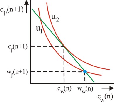
(6) cwh(n) + cph(n+1) × ρ(n) = wwh(n) + wph(n+1) × ρ(n)
The formula 6 is a straight line in the [cwh(n), cph(n+1)] plane, with a slope -1/ρ. It is depicted in the figure 2. It is clear that the household can reach each point on this line, simply by making the suitable choice of saving.
In the absence of savings the household h is in the point [wwh(n), wph(n+1)]. Since this is a point without any exchange, this is called an autarky9. Here the utility is Uh(wwh(n), wph(n+1)). The meaning of saving becomes clear, when the iso-utility curves of Uh = Uh(cwh(n), cph(n+1)) are considered, and these are also drawn in the figure 2. It is clear that the household h can increase its intertemporal utility by moving along the intertemporal budget line, until it is exactly tangent to an iso-utility curve. In that optimal point the intertemporal marginal substitution rate of cwh(n) and cph(n+1) satisfies10:
(7) MSV = dcph(n+1) / dcwh(n) = -(∂Uh(n) / ∂cwh(n)) / (∂Uh(n) / ∂cph(n+1)) = -1/ρ(n)
An interesting aspect of the figure 2 is also, that the effect of changes in the interest rate r(n) can be studied. For, they affect ρ(n), and thus the slope of the budget line (formula 6). It is obvious that a rising r(n) stimulates the households to save more, because thanks to the higher interest their consumption as pensioners will increase. The path that is followed in the [cwh(n), cph(n+1)] plane, when the interest rate rises, is called the supply curve of savings. It moves to the left and upwards.
Note that until now the argument about the OLG model has not yet used the discount factor δ. The intertemporal Uh(n) can still assume any form. However, interesting relations can be derived from the model, when one does posit the formula 2. Then it turns out that the consumption path can be calculated. Suppose that the consumptive utility equals u(c) = ln(c), then the formula 2 in the OLG model becomes
(8) Uh(n) = ln(cwh(n)) + δh × ln(cph(n+1))
Note that then exp(Uh(n)) has the Cobb-Douglas form. Suppose that the formula 8 holds for all households, with a single universal discount factor δh = δ. Furthermore, suppose that the economic system is in a stationary state. Such a state has the hallmark, that the variables do not depend on time. The production sphere remains the same, and thus also ww, wp, and r. Besides, it is assumed here, that the number of workers is constant in time, say H 11. Since the workers end as pensioners, the number of pensioners also equals H. Suppose that ww and wp are equal for all households. Now insert the formula 8 in the formula 7. The result is
(9) ρ(n) = δ × cw(n) / cp(n+1)
Eliminate cp(n+1) from the formula 6 with the help of the formula 9, then after some simple rewriting the result is
(10) cw(n) = (ww + wp × ρ(n)) / (1 + δ)
Combining the formulas 9 and 10 yields
(11) cp(n+1) = (ww / ρ(n) + wp) × δ / (1 + δ)
The formulas 10 and 11 together define the consumption path of the OLG model with discount factor.
Now consider the formula 3a for the clearing of markets, which is required in the Walrasian equilibrium. Since it is assumed that the number of workers and pensioners both are H, here the formula 3a reduces to
(12) cw(n) + cp(n) = ww + wp
The formula 12 obviously holds for the period n+1 as well. However, since cp(n+1) is prescribed by the formula 9, in this manner apparently cw(n+1) is also fixed. That is to say, the situation is characterized by a dynamic development of cw(n) with the time factor n. This dynamic development can be calculated, and then one finds12
(13) cw(n+1) = ww + wp × (cw(n) − ww) / (cw(n) × (1 + δ) − ww)
This shows that cw(n+1) indeed depends on the choice cw(n), and furthermore on the state [ww, wp] of autarky. Apparently there is a shifting consumption plan, which is accompanied by a change of ρ(n) in time. Now the requirement of a stationary state leads to the extra requirement, that the interest rate r is constant, and that cw(n+1) = cw(n) holds. The formula 13 shows that the state of autarky satisfies this condition. However, it will not maximize the utility. But there is a second stable state. Namely, compare the formulas 6 and 12. When ρ(n)=1 holds, and thus the rate of interest is r=0, then indeed the identity cw(n+1) = cw(n) will hold13. Such a path of stationary production and consumption is called the Golden Rule path.
The formula 13 is notably instructive, because it describes the dynamical behaviour outside of the stationary equilibrium. It represents the functional relation cw(n+1) = f(cw(n)). Since there are two stationary states, f(cw(n)) intersects the line(-function) cw(n+1) = cw(n) on two places. The reason is that, although it is true that f(cw(n)) is rising, it does so in a decreasing manner. Past the first intersection, at a certain moment ∂f/∂cw(n) < 1 will hold. This also implies, that between the first and second intersection one has f(cw(n)) > cw(n). Apparently in the dynamic situation cw moves from the lowest intersection towards the highest intersection, according as time progresses14. This has a remarkable consequence. Namely, when in the Golden Rule path the workers save, such as is depicted in the figure 2, then this path corresponds to the lowest intersection. And that is unstable. In this situation any positive disturbance of cw will move the situation dynamically into autarky.
The preceding text shows that discounting utility according to the formula 2 is a convenient manner for describing intertemporal choices in an economic system. However, the formula 2 is questioned by behavioural economics. The present paragraph summarizes several points of criticism15. An important objection is that especially in the short term people dislike to postpone the acquisition of a reward. However, according as the delay of payment concerns more the long term, they are less displeased. That is to say, the discount factor δ decreases rapidly in the short term, and falls just slowly in the long term. The discount rate d exhibits exactly the inverse behaviour. This can be included in the formule 2, by using the discount function D(n) = β×δn, with β<1. Merely for the first period n=0, D(0)=1 is chosen, so β=1. This D(n) is called the quasi-hyperbolic discount function.
Incidentally, when δ is not constant, then it is less meaningful. Perhaps, in such cases the discount function D(n) = (1 + α×n)-1 is a better alternative, with α a positive constant. For instance, α can be put equal to the discount rate d. For a given d, in the long run this function will fall less rapidly than δn. This is called hyperbolic discounting. It turns out that some laboratory experiments can be described fairly well with this function. The (quasi-)hyperbolic discounting takes into account, that people attach value to their immediate pleasure. Fortunately, people are aware of their lack of will-power, so that they can somewhat protect themselves against it. This is done by means of a conscious self-commitment in advance. This is explained analytically with the dual self model, where the individual is both principal and agent. The principal must conclude a convenient contract with himself as the unwilling agent.
An example of such a contract is to carry a small amount of money, when one expects to get into a situation with various seducive "bargains". Or one can even completely avoid a visit to places with such offers. That is conscious abstinence. It can be effective to delegate the execution to another actor, who is insensitive to seductions. This is called an external self-commitment. An undesirable side effect can be, that henceforth one can act less flexibly. Consider an action of citizens for raising the tax on smoking or alcohol.
When the state takes over the commitment, then there is liberal paternalism. An example is to restrict the sales of fireworks to just a few days. Another option is the cooling-off period, so that individuals can yet cancel an impulsive purchase. The social-security forces the workers to remit contributions, so that they are insured against various calamities. An old-age benefit is in fact forced saving. A variant is the default choice: the state supplies a public service in such a manner, that the general interest is prioritized, unless the citizen explicitely demands the alternative. For instance: everybody is an organ donor, except for the explicit refusers.

However, there are still other reasons, why the discount factor δ may not be constant. Worth mentioning is the mental book-keeping. The inclination to immediately consume strongly depends on the liquidity of the money source. For instance, an expenditure will be more easy with a credit card than with a savings account. Even having debts with a credit card is not considered as a problem. Perhaps the casino's use chips for this reasons. Incidentally, gains from games will easily be spent, because they are not considered as an income. Even professional investors are sometimes irrationally myopic and thus risk-averse. Investment-portfolio's are always diverse, sometimes without reason.
Small expenditures are made more easily than a single large one, for instance for durable consumer goods. This is the reason that automatically saving is so convenient. People prefer a purchase with trade-in, in the illustion that the trade-in yields extra money. On the other hand, people feel so uncomfortable under the burden of a debt, that they tend to pay it off too soon. It is clear that in all these cases the people have a rather irrational manner for discounting their intertemporal utility.
Finally, it is worth mentioning the preference of people for rising time series of incomes. Workers attach much value to a rising wage during their career. Even when a calculation with the formula 1 would show, that the present value of the wage sum over the entire life span is largest for a falling series, then the workers still prefer a rising series. Several explanations have been invented for this phenomenon. For instance, a rising wage is a form of forced saving: what one does not yet possess, can not be expended. A rising wage can give self-content, perhaps because people are very sensitive to differences. And the enterprises like to offer rising wages, because in this manner they address the income motive. For, an individual who expects wage rises, will make an extra effort not to get dissmissed.
Unfortunately the argument in this paragraph shows, that behavioural economics barely disposes of generally valid models. It offers merely in some cases a usable alternative for the theory of intertemporal discounting with δn. Behavioural economics is mainly empowering due to the image of man, that is sketched. The indivual is not a rationally calculating homo economicus, but a somewhat impulsive being with various emotional inclinations. It indeed raises the question to what extent it makes sense to try to explain the human actions by merely rational arguments. It is better to have no model at all than an unworldy model, even when the latter is a mathematical work of art.
The formula 2 makes the bold assumption, that the total utility U is a sum of separate utilities u(c(n)) in the N periods. This implies that the utility u(c(n)) in the period n does not depend on the utility u(c(m)) in the earlier period m. However, behavioural economics draws the attention to the fact, that people tend to get used to a certain level of prosperity16. They employ the consumption c(m) as a reference for their satisfaction with regard to a later consumption c(n). Due to this effect there is an intertemporal dependency between the utilities u(c(n)). The Dutch economist B.M.S. van Praag has studied the dependency, both theoretically and empirically. The present paragraph is based on his findings17.
Van Praag studies the utility (also called satisfaction) u(y(0)) due to an income y(0) in the period n=0. This utility is partly dependent on the situation of the household, such as the number of family members, the age, the profession, etcetera. The situation is registered in variables x1, x2, ..., in short in a vector x. However, the utility at n=0 is also dependent on the incomes y(n) in the preceding periods (n=-1, -2, ...). Besides, Van Praag assumes that the utility at n=0 is determined partly by the incomes y(n), that the household expects in the future (n=1, 2, ...). The reader be warned, that this deviates from the formula 2. Van Praag does not analyze the aggregated utility U of a time series, but the influene that the time series has on the utility u(y(0)) in a single period n=0! He wants to check how realistic the abstractions are, which are the foundation of the discounting with the formula 2.
Suppose that the household h must evaluate the utility of an income c(0) in the period n=0. Van Praag models this utility valuation with the help of the formula
(14) uh(c(0)) = αc × Σn=-NN ωh(n) × ln(yh(n)) + Σk=1K βc,k × ln(xk,h) + γc + εc,h
In the formula 14, αc, βc,k and wh(n) are constants, which characterize the income c(0). The ωh(n) weigh the importance of the period n, and are typical for matters of income. The boundaries -N and +N of the summation over n are in principle infinity. The model allows for K concrete factors, which determine the situation of the household in the period n=0. The term γc is a remainder for modelling the other factors of the situation. The term εc,h is a random variable, which models the deviations of the household with respect to the social norm, as expressed in the preceding terms of the formula 14. Readers who desire a more complete explanation can consult the previous column about the scaling of monetary utility.
The formula 14 is fascinating - just like many other findings in the work of Van Praag. Namely, it can be used for analyzing large-scale inquiries among households, and from this for calculating the social averages α, βk and ω(n). Here ln(y(n)) can be interpreted as the experienced or expected utility u(y(n)) of an income in the period n. These terms model both learning effects and possible preferences for the behaviour of the time series. In the same manner, the utility ln(xk,h) models the influence of various social situations on the preferences, which are entirely ignored in the formula 2. Macro-economics obtains a truly micro-economic foundation18.
Van Praag concentrates the remainder of his analysis on the ωh(n), which are a discount of the experienced or expected utility. However, the discounting concerns the intensity of the recollection of the utility, and not the loss in value by the shift in time (such as a delay)! This fundamentally distinguishes the weighing functions ωh(n) from the discount functions D(n). There does remain the assumption, that ωh(n) also decreases in value, according as n is further in the past or in the future. The immediate experiences and expectations dominate in the weighing of the utility alternatives uh(c(0)) 19. It is commonly assumed that ω(n) is identical for all households. However, Van Praag distinguishes the weighing functions according to the age τ of the main bread-winner, so that they obtain the form ωτ(n).
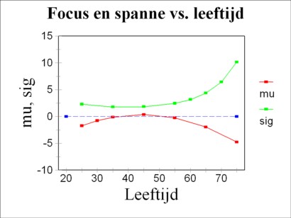
Van Praag has a natural preference for the normal probability distribution, and he also chooses her for modelling the distribution of ωτ(n) over de periods n. That is to say, ωτ(n) has the normal distribution N(n; μτ, στ), where μτ is the average of the distribution, and στ is the standard deviation. This choice is indeed somewhat subjective, because the form of the failing memory is not exactly known (no more than the discount functions D(n), which have just been discussed in this column)20. The two parameters μτ and στ are determined by means of a statistical analysis of data, in this case from the German socio-economic panel survey (in short GSOEP). Van Praag assumes, that they are polynomials of the second degree in τ. He calls μτ the time focus of the bread-winner, and στ his time span. The time span measures the disappearance from memory of experiences or expectations. A small στ implies that one lives in the moment.
In 1997 the participants in the GSOEP inquiry have answered the income evaluation question. That is to say, they have given their utility valuation for six incomes c. Van Praag takes 1997 as the period n=0, and thanks to GSOEP he disposes of sufficient data for summing in the formula 14 from n=-5 up to and including n=3 (the years 1992 up to and including 2000). Via xk,h Van Praag takes into account, among others, the family size for the whole time interval, as well as the age τ of the bread-winner for n=0. The figure 4 shows, that the time focus μτ and the time span στ change as a function of age τ. The result is really interesting. It turns out that middle-aged people live in the moment. And their time focus is slightly oriented towards the future. Conversely, the youth and the old people are lead by the past (due to μτ < 0). And their valuation is strongly influenced by the past and by expectations of the future21.
In any case the analysis of the GSOEP data shows, that the utility u(c(0)) of a present-day income c(0) is determined partly by the incomes y(n) in the past and in the future. Apparently the formula 2 is not very realistic. On the other hand, when it is abandoned, then also important findings such as the OLG model lose their foundation.