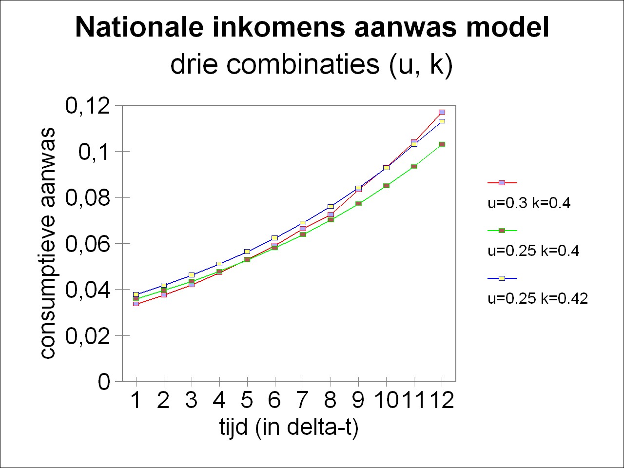
Figure 1: Consumptive growth for various u and k
Until now this web portal has paid much attention to the phenomenon of the economic growth. By doing so it has become clear, that it is possible to model growth. The economist Eva Müller explains that this can even be done at the level of the various productive branches, by means of the dynamic intertwined balance. However if one is only interested in the efficiency of the general economic development, then such models are too detailed. In those situations the dynamic one-sector models are more appropriate, because they are easier to handle. Notably the technological progress can be modelled in a fairly simple manner. Therefore they are often applied in the research of the long-term effects of the state policy. In such situations the one-sector models give an impression of the proportions between the national income N, the consumption K and the investments I, in connection with the technological progress. The optimal values of the various parameter can be determined by the method of systematic variation. The model calculations can provide predictions, they can support the proposed measures in a policy plan, or they can contribute to the analysis of policy. Thus the state is able to have some control over the national economy. The East-German economist Eva Müller presents in her book Volkswirtschaftlicher Reproduktionsprozeß und dynamische Modelle several of those models, and this column will describe two of them1. They are the national income growthmodel and the national income model, in its simplest version.
In principle both models are similar to the various growth models, that have been derived from the well-known economic theory of J.M. Keynes. However, Müller applies this theory to a system with central planning. This means that the propensity to save is a policy parameter. The central planning agency can optimize the amount of savings. In theory this is a huge advantage. Of course in practice it is dubious whether such an agency is really qualified and capable enough to make decisions concerning savings and productive investment.
Suppose that the national income is given by the function N(t), where t is the time variable. The foundation for the national income growthmodel is the equation
(1) ΔN(t) = k(t) × I(t-Δt)
In the formula 1 ΔN(t) is the growth of the national income during a period Δt. It has the mathematical form ΔN(t) = N(t) − N(t-Δt). The quantity I(t) represents the nett investments, that have caused the economic growth. Since evidently the investments must precede the growth, in the formula 1 their value for the preceding period must be inserted. The quantity k(t) is called the investment efficiency. She indicates the effect of various factors, notably those of the labour productivity (ap). As such she is a measure for the technological progress.
The investments in the production must be drawn form the national income, that is available at the moment. The remaining part, with an amount of K, is obtained by the households for their consumptive expenses. In mathematical notation this distribution is expressed as N(t) = K(t) + I(t). Of course the distribution is also apparent from that part of the national income, which has been added due to the growth. Since in the present column especially the growth is relevant2, the social distribution is formulated here by the relation
(2) ΔN(t) = ΔK(t) + ΔI(t)
Investments add capital goods to the already existing stock of equipment. It is a process of accumulation. Thanks to the accumulation more productive capacity becomes available, resulting in a larger size of the production3. The extra produced goods are divided according to the formula 2. The distributive code, that fixes the increase of the investments, can be written as
(3) ΔI(t) = u(t) × ΔN(t)
In the formule a u(t) is the distribution variable, which is called by Müller the rate of accumulation. It must be stressed, that the formula 2 is a relation between differences. In general she can not be made universal, in the sense that also the quantities themselves satisfy it. That is to say, normally I(t) / N(t) will not equal u(t).
The formulas 1, 2 and 3 together form the national income growthmodel. They suffice for the calculation of the changes in N, K, and I, provided that k(t), u(t) and I(0) are given. If one is interested in the absolute size of N, K and I, than also N(0) (or K(0)) must be known at the time t=0. That is to say, in that case the volume of N, and its distribution over the households and the productive sphere, must be determined in advance4.
The model is well suited for analysing the interaction between the accumulation and the technological progress. Müller describes on p.263 in her book how a systematic study was performed with regard to the economic development as a function of u(t) and k(t). Here the consumptive income K(t) is most important, because in the end it determines the observable wealth of the people. It is not surprising that a larger investment efficiency is favourable for the consumptive offer. The influence of the accumulation is more subtle, because she directly affects the consumptive share, and in addition according to the formule 1 she controls the growth of the national income. These two effects counteract each other.
The two-edged character of u(t) is illustrated by means of an example5. The initial conditions are N(0)=1 and I(0)=0.12. Both the investment efficiency and the rate of accumulation are kept constant in time. Three different combinations of u and k are considered, namely (u, k) = (0.3, 0.4), (0,25, 0.4) and (0.25, 0.42). The figure 1 shows in a graphic way how the consumptive income develops in time for each of the three combinations. It turns out, that at the start in the situation with u=0.3 the consumptive growth is the smallest. For a relatively large part of the national income is invested. But after 12 time steps of Δt the consumptive growth surpasses in this situation the growth in both other two combinations.
It is not a surprise that in the figure 1 the third combination, with a relatively large investment efficiency of k=0.42, yields a larger consumptive growth than the second combination. However it is not in advance self-evident that, such is appears from the figure 1, the third combination produces in the end less than the first one. Apparently in these three situations the rate of accumumation finally does settle the matter. Moreover the figure 1 shows, that the conclusions depend on the time horizon, that is used. Namely, only in the tenth time step does the growth in the first combination surpass the growth in the third one.
In the example the national income growthmodel has a fairly simple form. Thanks to the constant values of u and k an exact solution can even be found by means of infinitesimal calculus6. The practical importance of the model comes naturally to light, as soon as u(t) and k(t) represent time-dependent functions, which in reality is always the case. Further it must again be remarked, that the course of the curves in the figure 1 refers exclusively to the growth of the consumption. But it is evident, that a larger growth in the long run will by necessity also lead to a larger absolute consumption. The absolute consumption K(t) can be found by a cumulative addition of the growth ΔK(t). As a formula this is
(4) K(T×Δt) = K(0) + Στ=1T ΔK(τ×Δt)
In the formula 4 Σ is the well-known mathematical symbol for summation, in this case with a summation index τ. The consumption K(t) is visible in the figure 1 as the surface between the curves and the horizontal axis.
An important deduction from the calculations is that in advance the preferences of the people for present or future consumption must be gauged by means of opinion polls. If the people demand instantly more consumption goods, than austerity results for the investments. If on the other hand the people are willing to save for the future, then also the next generations will benefit.
The simple national income model distinguishes itself from the national income growthmodel by analysing the accumulated quantities N and K themselves instead of their changes. Moreover the economic growth is not coupled to the nett investments, but to the gross investments. These latter investments also register the deprecated equipment and its replacements. Hence the total stock of equipment enters as a variable into the formulas of the model. This variable G(t) is called by Müller the fundamental fund (in the German language Grundfonds) of the production. Here the equivalent of the formula 1 in the national income growthmodel becomes
(5) N(t) = g(t) × G(t)
In the formula 5 g is the efficiency of the fundamental fund.
The fundamental fund is described by the equation
(6) G(t) = G(t-Δt) + I(t-τ×Δt) + V(t-τ×Δt) − A(t-Δt)
In the formula 6 Δt is a time interval. The symbol I represents the nett investments, that is to say the installation of new, not yet available, production capacity. The investments expand G(t) with a delay τ×Δt, because some time elapses between the placement of the orders and the delivery of the equipment to the user. Nett investments can only be done, when capital is accumulated from the national income. In analogy with the formula 3 this is expressed as7
(7) I(t) = a(t) × N(t)
In the formula 7 a(t) is the rate of accumulation. Of course the amount of consumption is again that which remains, namely K(t) = N(t) − I(t).
The quantity V in the formula 6 represents the amount of replacements. The sum of I and V is the gross investment8. A replacement does not add new production capacity, but takes the place of the discarded equipment. It may be assumed that they are slightly more productive than the discarded equipment, simply because they are new, and thus do not yet suffer from defects due to wear. However the replacement does not employ new technology, for that would amount to nett investment. Nevertheless in practice a replacement will naturally be hardly equal to the discarded equipment. Also the replacements become available for the production process with a certain delay τ×Δt, because they must be manufactured after the placement of the order.
The quantity A represents the amount of discarded equipment. This is machinery, which can no longer be employed in the production process in a usefal way. The cause may be, that the equipment is worn, that is to say, its defects can no longer be efficiently removed by means of maintainance. It may also be, that the equipment produces end products, that are no longer in demand.
Note, that in the formula 6 only I(t) is an independent quantity. The other quantities A and V are an integral part of the existing fundamental fund G(t), because they keep up G(t) or reduce it. It makes sense to write
(8) V(t+(1-τ)×Δt) = v(t) × G(t)
and
(9) A(t) = w(t) × G(t)
In the formulas 8 and 9 v(t) and w(t) are respectivy the rate of amortization and the rate of discarding. So with d(t) = 1 + v(t) − w(t) the formula 6 can be rewritten as
(10) G(t) = G(t-Δt) × d(t-Δt) + a(t-τ×Δt) × N(t-τ×Δt)
The simple national income model can easily be applied, if it is assumed that τ=1. For in that case the formula 10 reduces to
(11) G(t) = G(t-Δt) × (d(t-Δt) + a(t-Δt) × g(t-Δt))
Now the model gives the solution in an analytic form. One has
(12) G(M×Δt) = G(0) × Πm=0M−1 (d(m×Δt) + a(m×Δt) × g(m×Δt))
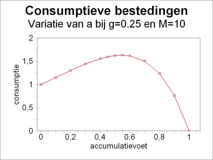
Figure 2: Consumptive expenses at different a
In the formula 12 G(0) is the initial condition, in other words, the value of G at the time t=0. The symbol Π has the usual mathematical meaning of a multiplication of the sequence of all M terms, from t=0 until t=(M−1)×Δt. Now N(t) can naturally be calculated from the formula 5. Subsequently K(t) can be found from
(13) K(t) = (1 − a(t)) × N(t)
This completes the formalism of the simple national income model. In essence it is of course the same as the national income growth model. However, the model has extra options, notably the time variation of the replacement and of the discarded equipment. In the model the dynamics of the fundamental fund of production is taken into account in a more realistic manner. Moreover now the efficiency of the whole fundamental fund changes in a persisting way, as a consequence of the formula 5, and not only the efficiency of the nett investments.
Eva Müller reports on p.269 v about a study of the effects of the parameters g, a and M in the model. It is assumed that they are independent of time. In addition v=w is assumed, so that one has d=1. Then the formula 12 gets the very simple form
(12) G(M×Δt) = G(0) × (1 + a × g)M
In this column now a single example will be given of this type of studies9. Suppose that N(0)=1 is given, as well as g=0.25 and M=10. Note that then one has G(0) = N(0)/g = 4. The figure 2 shows, how then the consumption K(10×Δt) varies as a function of the rate of accumulation a. Apparently the amount of consumption goods is largest for a=0.55.
Müller describes also the extended national income model10. In this version of the model there is no longer a single fund efficiency g, but various different efficiencies can be assigned to the nett investments, the replacements and the discarded equipment. Moreover next to these three efficiencies also the number of workers and their labour productivity can be introduced in the model. Taking it all in all, the model is more flexible. Evidently the disadvantage is that the number of parameters increases appreciably. According to Müller the statistical data are still lacking, that are needed in order to determine realistic values for all those parameters. Therefore your columnist forgoes the description of the extended version of the model.