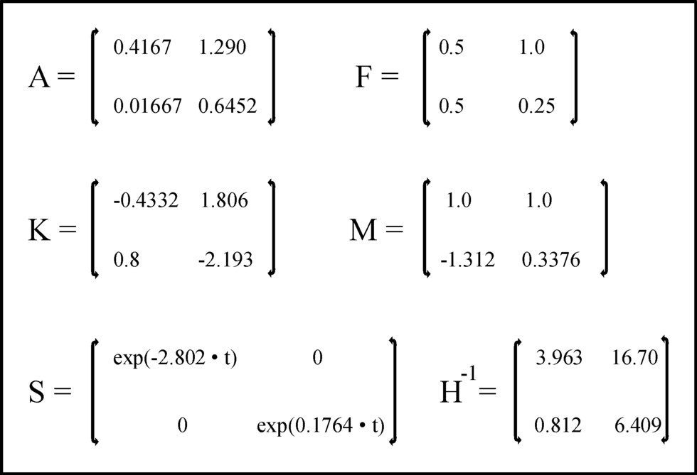
Figure 1: The elements in de matrices A, F, K, S, M and H-1
The phenomenon of the economic growth is one of the prominent scientific themes, because it directly influences our prosperity. Economists try to discover the conditions, that contribute to growth. An earlier column shows how the East-German economist Eva Müller expresses the dynamic growth model of Karl Marx in mathematical formulas. That column is followed by a second column, that shows how Sam de Wolff adds the technological progress to the growth model of Marx. The version of De Wolff is able to model the rise in the organic composition in the various economic branches. Both version are very suited for gaining insights into the effects of the economic proportions on the growth. However the presented economic system is rather simple, because they consist of only two (Eva Müller) or three (Sam de Wolff) departments. Besides in the scheme of Marx it is not immediately clear what sums are actually invested in the various branches. Müller must calculate the accumulation quotes separately by using the technical coefficients, and De Wolff uses even more complex methods for the calculation of the accumulation quotes.
In the neoricardian theory the economic system is modelled in an elegant manner by making use of matrix calculations. In its simplest form the model reduces to the open Leontief system, that describes how all product quantities xi(t) are related to each other. Assume that the system is able to generate at the time t a nett product ψi(t) in each branch. That nett product must satisfy the relation
(1) ψi(t) = xi(t) − Σj=1N χij(t)
In the formula 1 there are N branches, and Σ is the familiar mathematical symbol for summation, in this case over the index j. The symbols χij indicate the quantity of product i, that is needed for the production in the branch j. The set of numbers χij is called the intertwined matrix. Apparently in this context the quantities χij(t) play the role of means of production in all the production processes i. The χij mark the production technique, that is employed by the producer. In case that he would change to another production technique, the intertwined matrix should be modified accordingly. Only if the branch i produces more means of production than is needed in the N branchers, will there be a remaineder in the total nett product.
In the neoricardian theory it turns out to be useful to transform the intertwined matrix into the so-called production coefficients aij(t). They are defined by
(2) aij(t) = χij(t) / xj(t)
Substitution of the formula 2 into the formula 1 yields an interesting result:
(3) ψi(t) = xi(t) − Σj=1N aij(t) × xj(t)
This formula becomes even more succint, when the vector- and matrix-notation is employed:
(4) ψ(t) = x(t) − A(t) · x(t) = (I − A(t)) · x(t)
In the formula 4 A is the matrix with as its elements the production coefficients, and I is the unity matrix. Note that contrary to the neoricardian price equations the vector is placed on the right hand side of the matrix A. In other words, here x(t) is a vertical vector.
In the earlier column about the neoricardian theory only a static economic system is studied. Then the economy reproduces itself to all eternity. However, the formula 4 is quite suited for modelling the economic growth. To this purpose a method has been developed, that is called the fundamental model of the dynamic intertwined balance. This column gives an explanation of that model, that is presented by the economist Eva Müller mentioned just now1. Her presentation can be found in the book Volkswirtschaftlicher Reproduktionsprozeß und dynamische Modelle2. The starting point of the fundamental model is, that growth can only occur as long as there are investments in the extension of the means of production. It is assumed that the product technique remains unchanged. This implies that the matrix A is independent of time, that is to say, tne production coefficients are constants. Incidentally Müller calls the aij the coefficients of the direct material input (in the German language: Aufwand). Your columnist will follow her in this habit, simply in order to preserve the authenticiy of her argument.
In the study of the economic growth the quantity ψ(t) is especially important. For it contains the wages, as well as the profits and the taxes. These are the factors, that together determine the social prosperity. Then the formula 4 shows, that a growth of ψ(t) must increase also the total social product x(t). For the growth of ψ(t) removes a larger part from x(t), which then is no longer available as means of production. This skimming of x(t) must be compensated by its growth, not as a goal in itself, but just as the means to enlarge the richness. The size of the quantity is determined to a large degree by the fashionable techniques of the production processes. The part A · x(t) of x(t) will be consumed during the production, either as a part of the end product, or as energy or other resources, or as wear of the machinery and buildings. After each production cycle these quantities of products need to be again available in order to start the next cycle. Therefore Müller calls the part A · x(t) the material fund, in imitation of Marx. The term fund expresses that it is a permanent stock of goods3. Incidentally the material fund is also needed in the static neoricardian theory, although in that situation the fund does not expand.
The material fund consists of two components, namely in the terminology of Eva Müller the circulation fund and the basic fund4. The circulation fund covers all input of semi-manifactured products and raw materials, that are absolutely necessary for the generation of the end product, and that are partly integrated in it. The main mark of this input is the swift flow out of the production process, say with the completion of the end product. The basic fund guarantees that during the production process the durable means of production remain also available. This is the equipment, like machinery and the factory-buildings, that do not wear in a significant way. Marx calls this the fixed capital. In the case of economic growth, of course the production can only continue, as long as the basic fund expands as well. In other words, not just the circulating material input will increase, but the fund of fixed capital goods as well. In addition the basic fund supplies the means to replace the worn equipment. Incidentally the separation between the various forms of capital (circulation fund, basic fund) can be smooth. For instance oil as fuel is a circulating material input, whereas oil as a brake fluid is a fixed capital good, for in principle durable. And metal can be processed in the end product, but it can also be a durable part in the machinery.
The material fund must be replenished by means of investments i(t) 5. Of course they must come from the end product ψi(t), just like in the case of the reproduction schemes of Marx. Apparently the following separation of ψi(t) is useful
(5) ψ(t) = i(t) + y(t)
In the formula 5 y(t) is the nett product, that is available for the consumption, with the exception of the investments. Investments can be interpreted as a special type of consumption, namely in behalf of the material fund of capital goods. That is to say, thanks to the investments the fund is built up in the course of time. The wages must be paid from y(t), just like the profits and the taxes6. The nett product y(t) is merely consumptive, and is lost for the productive applications (even though of course for the workers the consumption is an existential condition).
Nett investments i(t) occasion a rise of x(t), because at the time t they add production capacity to the material fund. Investments always pertain to a certain time interval, for instance Δt. During this interval the expansion of the total product is x(t+Δt) − x(t). For a time unit this becomes (x(t+Δt) − x(t)) / Δt. One recognizes here the derivative of x(t), expressed as a difference equation. Investments can be made in a continuous manner, or intermittently. If the investments are continuous, then they can be represented by the formula
(6) i(t) = F · ∂x(t)/∂t
In the formula 6 F is a matrix with as elements the coefficients fij of the fund input. The fund input consists of the means of production i, that are present in the fund for the production of the good j 7. The elements fij are constants, that is to say, they are independent of the time. In fact the formula 6 is a linearization of the increase of x(t) in consequence of the investment i(t). This linearization is justified, because in the case of continuous investments the time interval Δt can be chosen arbitrary small. The formula 6 clearly shows, that a positive investment i(t) is a source term: it forces x(t) to keep growing. Although the formula does not elaborate on the causes of the growth, the preceding text has already drawn attention to the expansion of the material fund (production capacity).
Substitution of the formulas 5 and 6 into the formula 4 yields as result a set of differential equations, that describe the system:
(7) y(t) = (I − A(t)) · x(t) − F · ∂x(t)/∂t
In comparison with the neoricardian formula 4 the formula 7 contains an extra term for the fund input. Incidentally Eva Müller discusses in her book also two difference equations, in addition to this set of differential equations. In those cases the investment is applied intermittently. The present column is limited to the case of the formula 7 8. This formula completes the analytic modelling of an economy with an expanding production capacity and a nett product. The next step is the solution of the set9.
The explicit solution of a set of differential equations of the first order requires initial conditions, namely the value x(0) at the time t=0. But it does not suffice for the solution of the formula 7. For this is a set of inhomogeneous equations, and the solution can always be extended with a combination of solutions of the set of homogeneous equations. The set of homogeneous equations belonging to the formula 7 is:
(8) (I − A(t)) · x(t) − F · ∂x(t)/∂t = 0
First of all the homogeneous solution of the formula 8 is determined. It is immediately clear, that exponential functions satisfy the formula 8, that is to say, functions of the form:
(9) x(t) = m × es×t
In the formula 9 m is a yet unknown vector, that is independent of time. Substitution of the formula 9 into the formula 8 leads to
(10) (K − I × s) · m = 0
In the formula 10 the matrix K is defined as K = F-1 · (I − A). The index -1
For convenience the formula 11 is rewritten as a matrix equation. Note here, that mj can be viewed as a matrix M with elements mi,j. In addition Müller defines the matrix S, with elements δij × exp(sj×t). The symbol δij denotes the Kronecker delta, so that S only has non-zero elements on its diagonal. Using these new matrices M and S the formula 11 can be rewritten in the succint form
(12) x(t) = M · S · c
Now remains the task to find the particular solution for the set of inhomogeneous equations 7. Just now it was remarked that in this formula y(t) is the most interesting quantity. It makes sense to take the following form for y(t):
(13) y(t) = p × er×t
In the formula 13 p is a constant vector, that is to say independent of the time t, that remains to be determined. The quantity r is the rate of growth of the nett product, because one has Δy/Δt = r×y. A planning authority can use the formula 13 in order to prescribe the growth rate, that is desired by her policy. Then the required volume of production x(t) can also be determined. This is exactly the approach, that Eva Müller takes for the fundamental model of the dynamic intertwined balance.
The formula 7 is solved by means of the so-called method of the variation of constants10. In view of the formula 13 a suited trial solution appears to be
(14) x(t) = q × er×t
The vector q is independent of time and is calculated simply by substitution of the formulas 14 and 13 into the formula 7:
(15) q(t) = H-1 · p
In the formula 15 H is the matrix defined by H = I − A − r×F. Thus a particular solution of the formula 7 has been found. Then the general solution of the inhomogeneous set of equations takes the form
(16) x(t) = M · S · c + q × er×t
In fact the formula 16 represents a multitude of solutions, because the constant vector c can take on arbitrary values. The value of c can only be fixed by the initial condition x(0) on t=0. The formula 16 completes the fundamental model of the dynamic intertwined balance.
The construction of the solution in this paragraph is purely mathematical. The reader is warned, that the economic theory puts additional constraints on the method of solution. In any case x(t) and y(t) have to be positive for all times, because they represent quantities11. Also it would be unrealistic to have growth rates sj in the formulas 11 and 12, that are much larger than the growth rate r of the nett product. The additional requirements place a considerable limit on the number of acceptable mathematical solutions. This means notably, that for the given technique of production, belonging to the matrix A, the investments must be selected with care. That is to say, the choice of the matrix F of the fund input must more or less match A and r. It would be convenient to find the relation between A, r and F in a mathematical way. Unfortunately your columnist does not know how to do this.
As is usual, and in imitation of Eva Müller, the preceding model is illustrated by means of a calculation. The example is again the economic system with two branches, that has been described in the previous column about the neoricardian theory, and that thus is a good acquaintance for the regular reader12. Of course the difference with the then situation is that now the quantities depend on time. The first branch is agriculture, that is involved in the production of corn (measured in bales). The second branch is the industry, and she produces metal (measured in tons, that is to say, in 1000 kg). Both branches use a part of the produced corn and metal for themselves, as the means of production (in the shape of seed, fuel, equipment, and the like). Of course each branch employs workers. Their wages are paid in bales of corn (for bread, gin etcetera) and in tons of metal (for domestic appliances etcetera). To be precise, the branch of corn uses on a yearly basis χgg(t) bales of corn, χmg(t) tons of metal, and lg(t) workers. It produces xg(t) bales of corn on a yearly basis. Likewise the production factors of the branch of metal on a yearly basis are χgm(t) bales of corn, χmm(t) tons of metal, and lm(t) workers, and its production is xm(t) tons of metal.
In the fundamental model of the dynamic intertwined balance the two differential equations of the formula 7 must be solved. For that some data must be present, first of all the elements of the matrices A and F. If the nett product [yg(t), ym(t)] has the form of the formula 13, then in addition p (that is to say, the value [yg(0), ym(0)] on t=0) and the growth rate r must be known. And finally the solution of the first order differential equation requires, that the initial condition [xg(0), xm(0)] on t=0 is known.
The matrix A is copied simply from the example in the column about the neoricardian theory. For the sake of completeness he is shown again in the figure 1. According to the formula 6 the matrix F determines the volume of investments. The figure 1 shows the values of fij, that have been chosen in this example13. In imitation of the column about the neoricardian theory, [xg(0), xm(0)] = [12, 3.1] is taken as the initial conditions for x. The development of the nett product is determined in an unambigious way by the choice [yg(0), ym(0)] = [1, 0.3] 14 and r=0.1 Then the nett product, and with it the incomes, grow with approximately 10% per unit of time. Thus all data are present for the calculation of the sought development of the total social product x(t).
First the general solutions of the two homogeneous differential equations (formula 8) are determined. The solutions have the form of the formula 9. The parameters m and s are determined by means of the method in formula 10. Next the general solutions can be written as in the formula 12, where for the moment the constants [cg, cm] remain unknown as yet. In the following text these will be calculated from the initial condition x(0). Here a detailed presentation of the calculations is omitted, and just the results are shown. The figure 1 contains the elements of the matrices K, M and S.
Next the particular solutions of the two inhomogeneous differential equations 7 are determined. This solution has the form of the formula 14. The figure 1 presents the elements of the matrix H-1. With this also q is known.
The general solutions of the inhomogeneous differential equations are given by the formula 16. Now the constants[cg, cm] can be calculated from the initial condition forx(0). The result for the solutions xg(t) and xm(t) turns out to be:
(17a) xg(t) = 0.3912 × e-2.802×t + 2.634 × e0.1764×t + 8.975 × e0.1×t
(17b) xm(t) = -0.5133 × e-2.802×t + 0.8892 × e0.1764×t + 2.724 × e0.1×t
An interesting aspect of the formulas 17a-b is that with the progression of the time t the exponential power with the largest argument will become increasingly dominant. That turns out to be the middle term in the right-hand side of the formulas. Apparently in the long term the total social product obtains a rate of growth of 17.64%. This is larger than the rate of growth r of the nett product y(t), that is fixed at 10% by the central planning agency. Here two remarks can be made. First, apparently the central planning agency believes that the extension of the productive capacity as more important than the consumption. There are huge investments in the expansion of the production of the means of production.
And secondly, apparently in the long term the production in both branches (agriculture and industry) obtain the same rate of growth (17.64%), even though she deviates with respect to the nett product. Then the proportions in the production of the two branches become the ratio of the two middle terms, namely 2.634 / 0.8892 = 2.962 (bales per ton). One may remember, that on t=0 the production started with 12 bales of corn and 3.1 tons of metal, so with a ratio of 3.781. Appartently the proportions of production shift in favour of the industry. In other words, in this economic system the industry is involved in an overtaking manoeuvre, and grows faster than the agriculture.
The formulas 17a-b are not usable for negative times, that is to say, for the historical development of x(t). For then the first term on the right-hand side will dominate the other terms15. And as one sees from the formula 17b that term leads to negative quantities of xm(t).
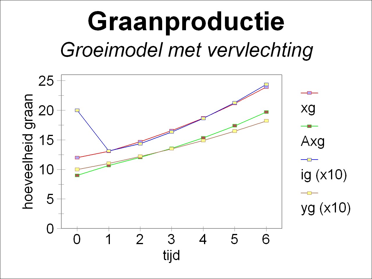
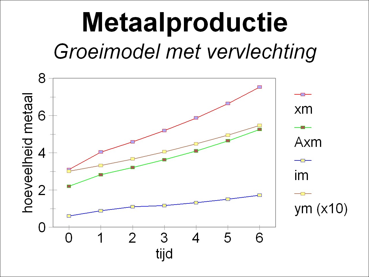
For the sake of completeness the table 1 shows the time development of the total social product (xg(t), xm(t)), of the material consumption (A · x(t)), of the investments (F · ∂x/∂t), and of the nett product (yg(t), ym(t)). The figure 2a-b shows the time development in an elegant way, for respectively the agriculture and the industry. Clearly visible is how the growth of consumption (the nett product y(t) without the investments) falls behind the productive growth. Of course the central planning agency can at all times decide to choose yet a larger r, if it desires so. It is again remarked, that in these suppositions the technology of production remains unchanged.
| time t | 0 | 1 | 2 | 3 | 4 | 5 | 6 |
|---|---|---|---|---|---|---|---|
| xg | 12 | 13.08 | 14.71 | 16.59 | 18.72 | 21.16 | 23.94 |
| (A·x)g | 9 | 10.66 | 12.05 | 13.60 | 15.37 | 17.38 | 19.69 |
| ig | 2 | 1.315 | 1.438 | 1.634 | 1.865 | 2.219 | 2.436 |
| yg | 1 | 1.105 | 1.221 | 1.350 | 1.492 | 1.649 | 1.822 |
| - | - | - | - | - | - | - | - |
| xm | 3.1 | 4.040 | 4.591 | 5.186 | 5.864 | 6.639 | 7.526 |
| (A·x)m | 2.2 | 2.825 | 3.207 | 3.622 | 4.096 | 4.636 | 5.255 |
| im | 0.6 | 0.8837 | 1.017 | 1.159 | 1.321 | 1.508 | 1.724 |
| ym | 0.3 | 0.3316 | 0.3664 | 0.4050 | 0.4475 | 0.4946 | 0.5466 |