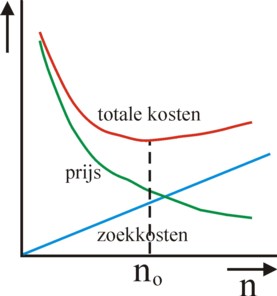
Figure 1: Optimal search behaviour
This column again presents several interesting models of new institutional economics. First the repeated game of the prisoners is analyzed. Next a model is presented, which takes into account the search costs on the market. Also useful are models, which describe the maintenance of norms. And finally the principal-agent model is again discussed. The used abstractions of human nature are tested with insights from psychology.
Traditionally the economic science uses the anthropology of the homo economicus: a rational decider, who defends his own interest. Moreover, in the standard theory he has stable preferences, and he is omniscient. This image of man is controversial, also within economics itself, since the rise of behavioural economics. Therefore during the past half of a century various new models have been proposed, which make the homo economicus more human. A large part of these models is included in the new institutional economics. It notably takes into account the transaction costs, which inevitably emerge during human actions. Such additional costs make the situation significantly more complex.
For instance, the complete search process for the optimal transaction itself is accompanied by costs. Moreover, investments are needed in order to maintain norms and other institutions. Labour contracts and other economic agreements are not automatically observed, so that extra costs are needed for their execution. On the other hand, a positive point is that under suitable conditions the homo economicus is willing to cooperate, albeit merely for serving his own interest. Nowadays such properties are included in the economic models, and the present column discusses some important ones.
In the present economic science the game theory has established a prominent position. In various columns the prisoner's dilemma has been mentioned. For the sake of convenience, this game (transaction) is presented in the table 1. There are two actors A1 and A2, who both can choose for cooperation or exploitation. They can not in advance make a binding agreement. The table 1 shows the rewards (b1, b2) for A1 and A2 in each situation1. It is clear that cooperation is the best option for the actors as a collective. However, each actor separately must fear, that the other will exploit him. In this situation each actor wants to optimize his utility (outcome). Therefore both actors will finally choose exploitation, although they thus obtain a bad result as a collective.
| A2 cooperates | A2 exploits | |
|---|---|---|
| A1 cooperates | 1, 1 | -1, 2 |
| A1 exploits | 2, -1 | 0, 0 |
The collectively worst outcome (0, 0) is called the Nash equilibrium. For, no actor can unilaterally improve his situation. And the choice of both actors is called the dominant strategy. In practice the one-shot prisoner's dilemma often occurs. However, even more often both actors will engage in repeated actions, and that changes the character of the game2. Namely, when the game is repeated, the actor must not optimize the one-shot outcome, but the outcome of all of his transactions together. It is interesting that A1 and A2 can use their transactions for mutually signalling their intentions. In the present situation it turns out that the tit-for-tat strategy yields good results. Both players start with cooperation, and in each subsequent transaction imitate the choice of the other in the preceding interaction.
It is immediately clear, that now both actors will always cooperate. Explotation by an actor would be foolish, because the other would imitate it. Incidentally, each actor could return to cooperation by again starting to do it. Explotation is no longer automatically the dominant strategy, because the tit-for-tat strategy can yield more for both actors. Under these circumstances the tit-for-tat strategy could become a social norm, which benefits all. Unfortunately the hallmark of an informal norm is, that not everybody observes it. Assume for the sake of convenience, that each actor separately and consistently chooses the tit-for-tat or exploitation strategy. One may calculate when obedience to the norm is profitable. Suppose that for each transaction the probability is π, that at least a further transaction will follow. The the total expected outcome is given by3
(1) Bk = Σj=1∞ bk(j) × πj-1
When one of the two actors is an exploiter, then after the first transaction both actors will exploit. This yields 0, so that the total expected outcome equals those in the table 1. The outcome will be different only when two actors in the tit-for-tat group meet. For, then one will always have bk(j) = 1. Therefore the series in the formula 1 obtains a simple form, namely 1 / (1 − π). The table 2 gives the outcomes of the repeated game of prisoners.
| A2 cooperates | A2 exploits | |
|---|---|---|
| A1 cooperates | (1 − π)-1, (1 − π)-1 | -1, 2 |
| A1 exploits | 2, -1 | 0, 0 |
Apparently the tit-for-tat combination leads to the best Bk, as soon as π>½ holds. Now suppose that a fraction p of the actors belongs to the tit-for-tat group. In other words, p is the trust, which the actor has in the validity of the norm. Then, according to the table 2 the expected outcome for the tit-for-tat strategy is p / (1-π) + (-1) × (1-p), and for the exploitation strategy 2×p. The tit-for-tat strategy is at least equal in value, as soon as p / (1-π) + p − 1 ≥ 2×p holds. That is to say, one must have p ≥ 1/π − 1. This formula expresses the quality of the norm. A special case occurs, when an (almost) endless series of transactions is expected. For, then one has π=1, so that p≥0 must hold and therefore the actors with a tit-for-tat strategy perform on average as good as the rest, or better.
Remarkable is also the situation, where two actors do adhere to the tit-for-tat norm (that is to say, p=1), but on j=J+1 by accident one chooses exploitation. Suppose that the last interaction occurs on j=N (which is evidently unknown in advance). Tit-for-tat implies, that the reaction to the action of the other is lagged. Therefore, now for interactions j>J both actors will alternate exploitation and cooperation, which results in a series of outcomes (-1, 2) en (2, -1). Then one will have Bk = J×1 + (N − J) × ½ × (-1+2) = ½ × (N+J). The mistake of the one actor has caused a loss of no less than ½ × (N-J) for both. Apparently the other actor will benefit from forgiving the mistake, and continuing to cooperate. That would yield N-2 for him, and N+1 for his clumsy competitor. The tit-for-tat strategy would no longer by optimal4.
This example of the prisoner's dilemma with repetition makes the essential assumption, that the actors have a fixed strategy. They are encouraged in their morals by the fact, that the moment of the last interaction is unknown. Only in this case the tit-for-tat strategy is interesting. For, suppose that j=N would with certainty be the last interaction5. Assume furthermore, that the actors have yet to choose their norm of stategy. In the interaction j=N, exploitation becomes again the dominant strategy. However, now it follows, that the tit-for-tat strategy is also unsound for j=N-1. Therefore on j=N-1 the strategy of exploitation also dominates. Etcetera. Rational actors will already immediately at j=1 select exploitation as their norm. Apparently the tit-for-tat strategy is only rational for an undetermined repetition of interactions. Fortunately in reality the number of interactions is usually indeed indeterminate in advance.
In conclusion: as long as the number of interactions is indeterminate, a certain norm of behaviour will not develop naturally. It is true that for a sufficiently large p it is optimal and thus rational to adhere to the tit-for-tat morals. But when an actor prefers the morals of exploitation, then this is a stable situation, where cooperation will never occur. Nevertheless, experiments in laboratories show, that the test persons indeed exhibit some tit-for-tat behaviour. Incidentally, the situation can develop in a dynamic manner6. Furthermore, in such experiments it turns out, that even in one-shot games or transactions the actors are sometimes inclined to cooperate. Apparently man is by nature not a homo economicus, who purely egoistically and rationally defends his own interest7. Besides, certainly outside of the laboratories the individuals are socially embedded, and subjected to group pressure, so that it becomes rational for them to moderate their own egoism8.
The famous economist R.H. Coase has emphasized the search costs, which must be made in order to find the best product-price combination on the market. The search naturally does save money, because in this manner the actor realizes a favourable exchange. This implies, that an optimal search-effort exists, where the benefits and the costs of the search are balanced. It is possible to describe this search behaviour by means of a mathematical model9. Suppose that the distribution of prices p is uniform in the interval [0, pmax]. That is to say, the distribution function (probability density, frequency function) has the constant value f(p) = 1/pmax. Let F(p) = ∫0p f(ρ) dρ = p / pmax be the cumulative distribution function. It is the probability that the supply price is not larger than p. Apparently there is a probability of Pr(>p) = 1 − p/pmax, that the supply price is higher than p.
The search of the consumer requires demanding various offers (unless the first offer is a fortunate random hit). Namely, according as one has more offers, it becomes more probable that it includes a low offer. Suppose that the isolated demand of an offer leads to costs c, and that the consumer wants to buy q pieces of the product. Suppose that the lowest supply price of all those n offers is at most p0(n). Unfortunately the consumer can not in advance calculate his final costs T, due to the random nature. But he can estimate the expected costs, namely E(T) = E(n×c + q×p0) = n×c + q × E(p0). The minimization of E(T) is only possible, when the relation between the expected E(p0) and n is determined.
Assuming n offers, all offered prices are p0 or larger with a probability of Pr(>p0)n. It follows immediately from this, that the situation, where at least one offered price is below p0, occurs with a probability of 1 − Pr(>p0)n. This probability Pr(p ≤ p0) naturally corresponds again with a cumulative distribution-function, say G(n, p0). The corresponding density-function g(n, p0) is the derivative of G. Thus p0 has the expected value10
(2) En(p0) = ∫0pmax p0 × g(n, p0) dp0 = pmax / (n + 1)
Now the consumer can determine, when demanding the next offer is no longer profitable. According to the formula 2 the expected costs E(T) are minimal for n = -1 + √(q×pmax/c). Therefore this is the number of offers, that is optimal for the consumer (see figure 1). This value n=n0 also determines, by means of the formula 2, which upper limit p0 of the supply price is desirable for a given c and q. There is truly an exchange possible between information costs and the sales price. The consumer may of course have bad luck, so that after n offers all supply prices are still above p0. On the other hand, he may be lucky, and (almost) immediately obtain a low offer. In this case it is useless to continue the search. There are rules of thumb also for this situation11.
For, let p0 be the unexpectedly low offer. Demanding another offer only makes sense, when it is expected that this transaction will lead to lower costs than q×p0, so that E(T, another) = c + q × E(p, another) ≤ q×p0. Now E(p, another) has two components. The next offer can lie above p0, with a probability of Pr(>p0) = 1 − p0/pmax. In that case the sales price remains p0. Or the next offer lies below p0, and then one has E(p0') = ∫0p0 p × f(p) dp = p0²/2. Combining the two components yields E(p, another) = p0 × (1 − ½×p0/pmax). Insertion in the formula for E(T, another) leads to
(3) E(T, another) = c + q × p0 × (1 − ½ × p0/pmax)
Apparently another search offers good prospects, as long as one has c ≤ ½×q × p0²/pmax. This model surprisingly shows, that the neoclassical paradigm can take into account the transaction costs. Here it must be noted, that the situation is special. For, the consumer knows in advance the probability distribution f(p) of the supply prices. This is also information, which undoubtedly came with a price for the consumer.
For instance, he may be a member of a consumer network, which provides him with information. According to the theory of social capital Cs such networks can indeed reduce the transaction costs. The members of a network pay a price, namely that they must maintain the collective norms of the network, by being obedient and by encouraging others to adapt. Besides, the members of the network will only cooperate, for instance by providing information, as long as the beneficiary feels obliged to return the favour at a later time. Such complex mechanisms can not be included in the model. The neoclassical paradigm does not (for the moment) contain formulas to describe social processes such as rights and duties. Therefore many still feel somewhat discomforted, when applying this paradigm.
At the end of the preceding paragraph is has been suggested, that each group has its own informal and formal institutions. These make the individual behaviour easier to predict, but also limit the freedom of the group members. Institutional influences are important, but their theoretical modelling is yet in its infancy. A previous column has described some of these early models. The present paragraph elaborates on this. First, consider the game of Tsebelis, which models the interaction between a group member A1 and an inspector A2. The group member A1 can obey the group norm, or violate it. The inspector A2 can maintain the norm, or fail to do this (for the love of ease or another reason). The table 3 summarizes the typical outcomes of this game12. The reader can check, that the outcomes are logical. For instance, as long as A1 obeys, it does not make sense for A2 to maintain.
| A2 maintains | A2 does not | |
|---|---|---|
| A1 violates | 0, 1 | 1, 0 |
| A1 obeys | 1, 0 | 0, 1 |
This game is special, because there does not exist a Nash equilibrium of behavioural strategies. For, each outcome (b1, b2) allows one of the actors to improve his situation by changing his behaviour. For instance, suppose that A1 obeys, and A2 does not maintain. Then A1 benefits from henceforth violating the norm. This situation is confusing for both actors. In principle they can create a Nash equilibrium by both choosing a so-called mixed strategy. For instance, A1 can choose to obey with a probability of p1, and therefore to violate with a probability of 1 − p1. In the same way A2 must choose to maintain with a probability p2, and therefore to fail to do it with a probability of 1 − p2. The matrix of probabilities is shown in the table 4.
| A2 maintains | A2 does not | |
|---|---|---|
| A1 violates | 1-p1, p2 | 1-p1, 1-p2 |
| A1 obeys | p1, p2 | p1, 1-p2 |
In such a situation with mixed strategies the outcomes are purely coincidental, so that the actors can merely estimate the expected outcomes E(bk) for a series of interactions. Thus one finds E(b1) = p1 × (p2×1 + (1-p2)×0) + (1-p1) × (p2×0 + (1-p2)×1) = 2×p1×p2 − (p1+p2) + 1. Now A1 obtains his best outcome for ∂E(b1)/∂p1 = 0, that is to say for p2=½. In the same way one has E(b2) = p2 × ((1-p1)×1 + p1×0) + (1-p2) × ((1-p1)×0 + p1×1) = p1+p2 − 2×p1×p2. Also A2 obtains his best outcome for ∂E(b2)/∂p2 = 0, that is to say for p1=½. Apparently it is attractive for both actors to choose the mixed strategy with p1 = p2 = ½. The expected outcome in this optimum is (½, ½). The situation is comparable to the best reactions in an oligopoly of the Cournot type. An actor, who deviates from this, hurts himself and favours the other. An example: for p2=¼ one has E(b1) = ¾ − ½×p1. Then A1 can choose p1=0 and the outcomes are (¾, ¼).
Thanks to the mixed strategy now a Nash equilibrium can be realized. The two actors have created a stable situation in a rational manner. In addition, there is predictability, at least concerning the average behaviour. However, it would imply that the actors no longer use a pure-strategy norm, which intuitively feels undesirable. The human nature and cognition are not designed to apply morals in an opportunistic manner. This illustrates that indeed sometimes the instrumental rationality is less appealing than value rationality. Nevertheless, in practice the mixed strategy yet often occurs. Consider the inspection of passenger tickets in the public transport, which is never more than taking regular samples. Yet the intention is also here, that free riding is discouraged, and that the passengers internalize the norm .
The internalization of institutions is a fascinating theme, because in this way the individual changes his utility function. The Dutch economist P. Frijters has made a first attempt to include this phenomenon in the utility function. His colleague B.M.S. van Praag has found empirical formulas for the preference drift, where the individual adapts the utility to his reference group. Nonetheless the majority of the models assumes a fixed utility function. Then the individual is simply a rational decider. Consider again an actor A1, who expects an outcome b1 of a transaction. This yields him a utility v(b1). Suppose that he can increase the outcome with Δb1 by violating a norm. This would make the transaction more useful. Unfortunately for A1 there is an inspector, who can punish violations with a fine s. Just like in the game of Tsebelis the probability of maintenance equals p2. Then the expected utility U of A1 due to a violation becomes13
(4) U = p2 × v(b1 + ρ×Δb1 − σ×s) + (1 − p2) × v(b1 + Δb1)
The parameters ρ and σ have values between 0 and 1. That is to say, even in the case of maintenance it is conceivable that A1 yet appropriates a part of Δb1. For instance, the inspector will sometimes not know the true size of Δb1. Conversely, it is conceivable, that the fine s is not imposed completely. For instance, A1 can have good relations with lawyers. Or A1 simply underestimates the sanction s by a factor σ. Finally, assume that the actor A1 is neutral to risk. Then he will decide to obey the norm, as long as one has U ≤ v(b1). Therefore the inspector must choose the parameters p2, ρ and σ in such a way, that this condition is satisfied. It follows immediately from the formule 4, that A1 will obey as long as one has
(5) p2 ≥ (v(b1 + Δb1) − v(b1)) / (v(b1 + Δb1) − v(b1 + ρ×Δb1 − σ×s))
The formula 5 shows, that the inspector has several options. A reduced probability p2 can be compensated somewhat by increasing the fine s. Due to the neutrality of A1 with regard to risk it can be assumed that v(b) = b. Write the right-hand side of the formula 5 as p2°. Then one has p2° = 1/ (1 − ρ + σ×s / Δb1), and the elasticity of p2° for s can simply be calculated: (∂p2° / ∂s) × (s / p2°) = -p2° × σ×s / Δb1.
The formula 5 is useful, because it clearly shows the causal relations for maintenance. Nevertheless, it is difficult to apply in practice. For, each individual has his own utility function U. Some will not be risk-neutral, but avoid or search risk. Those who can bearly live from b1, will have a strong desire to acquire Δb1. Sometimes an offender can count on the admiration in his own subgroup14. It turns out the children are more stimulated to internalize a norm, when the punishment s is mild instead of severe. Since the external coercion remains limited, they get the idea that obedience to the norm is a personal choice15. And since the function U is so personal, this model has mainly been applied to statistical data of large groups, where the individual properties average out.
Furthermore, note that the fine s can also be immaterial. Think about loss of status, disapproval by the group, or even exclusion16. In fact the immaterial punishment will even dominate within groups, because most group norms are informal. For, violations undermine the mutual cohesion, and therefore the existence of the group. Moreover, obedience leads to self-affirmation of the group members, so that conversely a violation can be accompanied by some self-punishment17. The differences in power between the group members originate more from the social relations than from the material inequality. The immaterial sanctions naturally cause material losses in the long term, but the size of those losses is difficult to quantify. The rational-choice paradigm of the sociologist J.S. Coleman is a couragious attempt to model the exchange (substitution) of material and immaterial sanctions.
A core piece of the new institutional economics is the principal-agent problem. A well-known variant of this problem is the situation of an enterprise, which due to several accidental circumstances has a fluctuating production q per period of production. That is to say, q is distributed according to a probability density f(q). The variant assumes, that the yield q is completely spent on paying the wage sum w and the profit π (so q=w+π). Therefore the income of the participants in the enterprise is subjected to risk. Suppose that the workers (as agents) are risk-averse, whereas the entrepreneur (as principal) is risk-neutral. In this situation it is important, whether the entrepreneur is able to measure the effort e of the workers. When this is the case, then the wage can simply be fixed in a contract. But when the entrepreneur can not measure e, then he must include income incentives in the labour contract.
It is common in this variant to mathematically calculate the optimum of the entrepreneur and the workers. However, it is also possible to analyze the problem by means of an Edgeworth box, and that is the theme of this paragraph18. Although the graphical method does not yield new knowledge, it does deepen the already existing insights of the mathematical method. The Edgeworth box is usually applied in the description of the exchange of goods. Here a special exchange will by analyzed, namely the distribution of the income risks. The application of the graphical method requires, that the probability density f(q) of the yield is simple. Only two yields are allowed, namely qH with a probability of pH, and qL with a probability of pL = 1 − pH, where qH>qL holds. Then the income risk is qH − qL. It is advantageous for all, when the entrepreneur insures his workers for this risk, and in exchange receives a contribution19.
The figure 2 shows the Edgeworth box for the insurance. Horizontally the incomes for qH are displayed, and vertically the incomes for qL. The origin of the coordinate system (wH, wL) of the workers is left below, and the values along the axes increase to the right and upwards. The origin of the coordinate system (πH, πL) of the entrepreneur is right above, and the values along the axes increase to the left and downwards. So the origin of the entrepreneur is the point (qH, qL) of the workers, and vice versa. Since the workers value security, they prefer the situation wH= wL. In the figure 2 this so-called certaintly line is shown as the line with an angle of 45°. For the sake of convenience the certainty line of the entrepreneur is also shown. These two lines coincide only, when qH=qL holds.
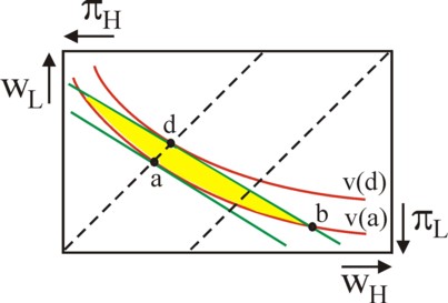
The expected wage of the workers is E(w) = pH×wH + pL×wL. A similar formula holds for the expected profit E(π). In the figure 2 the lines with a constant expected income (E(w)=a or E(π)=a with constant a) apparently have a slope of -pH/pL. Call these the iso-wage lines (for the workers) and the iso-profit lines (for the entrepreneur). Note that E(w) + E(π) = E(q), and this is fixed in the present situation. Therefore the iso-wage lines and the iso-profit lines coincide. In the figure 2 they are shown in green. The workers derive an utility v(w) from their wage, and the entrepreneur experiences an utility φ(π). Since the entrepreneur is neutral to risk, the indifference curves (φ(E(π)) = φ(a) = constant) of his expected profit match his iso-profit line E(π)=a. Therefore both are shown as green lines in the figure 2.
This is different for the workers. Consider an iso-wage line E(w)=a. In the intersection with the certainty line E(w) = wH = wL one has v(E(w)) = v(a). Yet the indifference curve v(E(w)) = v(a) of the expected wage does not coincide with this iso-wage line. For, when one moves over the iso-wage line, in such a manner that the distance to the mentioned intersection increases, then the difference wH − wL becomes larger and larger. This leads to dissatisfaction for the workers, which decreases their utility v. The workers want to have a material compensation, as it were, for the extra risk. The graphical expressions of this risk-aversion is the convex indifference curve v(E(w)) = v(a), which is shown in red in the figure 2.
The figure 2 also shows the consequences of the various risk preferences for the labour contract. Let the point b = (wH, wL) be the original contract. That contract is not optimal. For, the indifference curves of the workers and the entrepreneur, which intersect in b, separate outside the point of intersection. The largest distance between two indifference curves is reached on the certaintly line of the workers, namely the length of the line-piece a-d. The points a and d are also the points of contact of the indifference curves of the entrepreneur with those of the workers20. In the point a the entrepreneur has increased his utility in comparison with the point b. The same holds for the workers in the point d. Each of these contracts insures the workers against wage fluctuations. The relation of power will determine which of these points will be selected21.
Note that each contract in the yellow area of the figure 2 is better than the original contract in b. The relation between the principal and the agent becomes more complicated, when the principal must make costs in order to measure the effort of the agent. Suppose for instance, that the probability pH depends on the effort e of the workers. That is to say, one has pH = pH(e), with evidently ∂pH/∂e > 0 and thus ∂pL/∂e < 0. The entrepreneur wants to stimulate the efforts, because they increase his expected profit E(π). Unfortunately he can not determine e from q, because each qH or qL is due to a random process. The attitude of the workers towards e is ambiguous, because they experience the effort as a burden. Let c(e) be the size of the burden (costs, dissatisfaction). In this situation their utility is given by
(4) u(w, e) = v(w) − c(e)
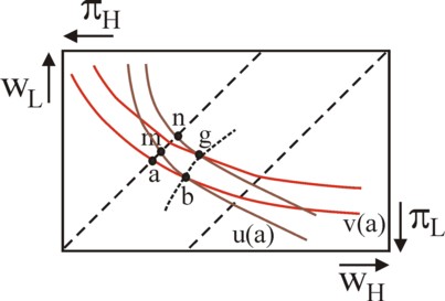
Thus the workers try to maximize w and minimize e. When E(q(e)) increases, then the entrepreneur can indeed pay higher wages w(e). The workers know the motives of the entrepreneur, and can exploit them by telling lies about their effort22. This forces the entrepreneur to determine the circumstances, where the workers will truly (of their own free will) make an extra effort. His method is explained in the figure 3. The indifference curves v(w) of the figure 2 are also shown here. Assume that on these curves e is not experienced as a burden, so that c(e)=0 holds. Now suppose that the workers will decide to make an extra effort Δe. This will create new indifference curves, which in the figure 3 are presented in brown. The new indifference curves are steeper than the old ones, because Δe raises the ratio pH/pL and therefore the iso-wage lijn will be steeper.
The figure 3 shows two points of intersection of the old and new indifference curves, namely b and g. First consider the point b, defined by v(E(w)) = v(a) = u(E(w), Δe). The new indifference curve through b intersects the certainty line in the point m. Note that without the extra effort this point would correspond to a larger utility v(m). The formula 4 shows, that the difference v(m) − v(a) is exactly the burden c(e + Δe) of the extra effort. Apparently on the new indifference curves the workers receive a higher wage w 23. Therefore the workers are tempted to state wrongly that they have made the effort Δe. Fortunately, this is different in the part of the new indifference curve u(E(w), Δe) = v(a) below b. For, this part is below the old indifference curve. Without the extra effort the points of this part have a utility v(w), which is lower than v(a). Now the workers are willing to voluntarily make the effort Δe.
The same argument can be applied for the point g, and for all other points on the dotted curve. On the right-hand side of the dotted curve the entrepreneur can be confident, that his workers will indeed supply the contracted e. In short, the entrepreneur must take care, that he does not offer labour contracts on the left-hand side of the curve b-g24. This is elaborated in the figure 4.
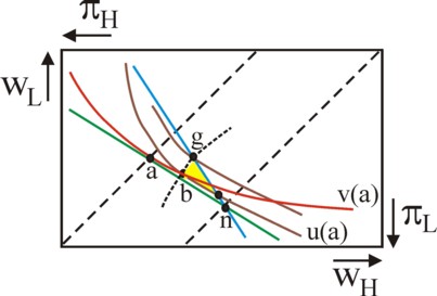
Suppose, the point a represents the old labour contract without extra effort. Here the wage is w=a, so that the iso-profit line is given by E(π) = E(q) − a. This is also the indifference curve φ(E(π)) = φ(E(q) − a) = constant of the entrepreneur (green line). It intersects the certaintly line of the entrepreneur in the point n. In the situation with extra Δe the new iso-profit line and indifference curves of the entrepreneur become steeper. The blue indifference curve in the figure 4, through the points n and g, is an example of this. As already stated, it corresponds with a constant utility value of φ(E(q) − a). However, above the line a-n the old indifference curves have a value below φ(E(q) − a). Apparently Δe indeed favours the entrepreneur. Thanks to the extra effort better labour contracts are possible than a, namely the points between the old and new indifference curve.
The entrepreneur must focus on the better contracts on the right-hand side of the curve b-g, due to the opportunism (exaggerate the effort) of the workers. Moreover, the workers do not want to give up utility, so that those contracts must lie above the new indifference curve u(E(w), Δe) = v(a) of the workers. Thus one finds in the figure 4 the feasible improved contracts in the yellow area. The concrete choice of the contract again depends on the power relations. It is striking that the contracts no longer lie on the certainty line of the workers, so that they are now willing to bear some risk. The unobservable value of Δe blocks an exchange, which would yield the optimal distribution of the risk. Therefore on the curve b-g the indifference curves of the workers and the entrepreneur do not touch. Incidentally, the contracts do satisfy Pareto efficiency.
Another interpretation of the situation is, that the workers must get an extra reward in order to compensate them for their income risk. This clause in the contract is unfavourable for the entrepreneur, because he is risk-neutral and therefore would be willing to bear the risk of the workers against lower costs. The necessity to pay a premium to encourage the workers (the limitation of the feasible contracts due to the curve b-g) makes this spread of risk unfeasible. This would obviously change, when the workers become risk-neutral. These conclusions are found in the preceding column about the principal-agent problem with unobservable effort. Graphically oriented readers will undoubtedly prefer the derivation in the present column25.
It is stressed again that this model sketches an abstract picture of the labour contract. In reality the entrepreneur disposes of many additional instruments in order to motivate his workers. These instruments are often based on some trust between the entrepreneur and his workers. The appreciation for justice and reciprocity are a part of human nature. These are called prosocial norms. Mutual obligations are exchanged for the long term. Nevertheless, your columnist still believes, that the homo economicus of the hedonistic wage-theory is a plausible anthropological model and that the presented principal-agent model contributes to the insight.