Decomposition and dating of quantities in the production

First insertion on Heterodox Gazette Sam de Wolff: 22 april 2013

Various preceding columns have presented discussions of production models, that use intertwined matrices (sometimes called Leontief models, input-output tables, or balances). The present column describes methods for the calculation of the material coefficients of the total or full input (in the German language Bedarf, Aufwand) in the production. Besides, a method is presented for the dissection of prices into quantities of dated labour. These methods are useful for the economic planning at the macro level.

In this column several simplifying assumptions are made. The producers dispose of a single existing production technique. The techological progress, and thus the innovation, is ignored. Therefore, the growth due to a rising productivity of labour is ignored. Moreover, the presented calculations are limited to linear production models. Consequently the possible positive effects of scale are ignored. Here a rise of scale will not change any proportion in the production. The common expression for this neutral situation is constant returns to scale.

In fact the column is completely based on the book Vorlesungen zur Theorie der Produktion by the famous economist Luigi L. Pasinetti¹. But the motivation to write the column has another origin, namely the many economic works from the former Leninist block. In these states the production models were popular, because they give insight in the functioning of planned economies. At the time the Eastern European governments have invested much in research, that tried to make the models applicable for the economic practice. The column will on several locations refer in footnotes to the Leninist literature, which your columnist has acquired notably from the Berlin second-hand bookshop Helle Panke².

It is unfortunate that this rich source of literature had been ignored by the west. There are several reasons. First, the free market economy can not be reconciled with a central plan. Incidentally, here the scientific institutes can not even access the information about the production of the enterprises. Second, there was an ideological barrier: all Leninist products were supposed to be inferior. And third, most of the literature was published in the Russian language, which was never popular in the west.

The total or full input in the production

In the column about the intertwined balances the fundamental equation of the neoricardian theory has been defined³

(1)     y = (I − A) · Q

Contrary to the mentioned column now the time variable t will be left out, because the present column only considers static situations. The formula 1 is a vector equation in n dimensions, where each dimension corresponds with a branch of economic activity. Each branch generates only a single product. The quantities in the total product are represented by the vector Q. The vector y is the end product, or according to Sraffa the nett product.

The difference term I-A shows that the end product is smaller than the total product. Here I represents the unity matrix, and A is the matrix with elements a_ij = q_ij / Q_j. The indices i and j lie in the interval 1...n. The symbol q_ij expresses the quantities of product i that are needed in order to generate a quantity Q_j of the product j. The elements of A are called production coefficients in the western states, whereas in the Leninist states they are called the coefficients of the direct material input or the coefficients of the circulating input (in the German language Q_j)⁴.

Apparently in the production coefficients the required quantity q_ij is reduced to the quantity per unit of j. This is expressed clearly in the formulation ∂q_ij/∂Q_j = a_ij. Furthermore, note that the index j refers to both the branch and its product. The formula 1 expresses that a part of the total product is consumed by the branches themselves.

If desired the formula 1 can be supplemented by a relation, which describes the connection between the size of the production and the required amount of labour. In vector notation the relation is

(2)     L = a · Q

In the formula 2 L is the totally required amount of labour. The right-hand side is the inner product of two vectors. The vector a consists of the components a_j = l_j / Q_j, where l_j represents the required quantity of labour in the branch j. In other words, the vector represents the quantity of labour which is required in the branch j in order to generate a unit of the product. The components of a are also called the coefficients of the direct input of labour, or in short the labour coefficients. Together with the production coefficients they form the technical coefficients.

Identify the inverse matrix of I-A by the symbol B. Then the formula 1 can simply be rewritten as

(3)     Q = B · y

The elements of B are represented by β_ij, and they are evidently constants as well. Apparently the coefficient β_ij expresses the quantity of the product i, which must be generated in total for a unit of the end product j. She can be written by means of mathematics in the form of the partial derivative β_ij = ∂Q_i/∂y_j. In other words, she is the totally required quantity of means (in the German language: the Bedarf) for the production of the final consumption. She contains, in addition to the direct material input (the means of production A·Q), also the indirect material input.

In the Leninist states the β_ij were called the coefficients of the full input⁵. The formula 3 can be considered to be the foundation for planning, because the plans are commonly based on the end product. The size of the economic system is merely its derivative.

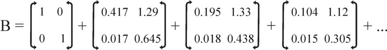
In the matrix theory it can be proven, that the matrix B equals I + A + A² + A³ + ... ⁶. Substitution of this power series into the formula 3 yields

(4)     Q = y + A · y + A² · y + ...

The formula 4 is a dissection of the total product Q in such a manner. that the production structure is clearly visible. First the production system must generate the end product y. But this does not suffice. The production of y can only proceed, when a quantity A·y of the means of production is available. That explains the second term in the right-hand side of the formula 4.

Figure 1: Production layers in the production of metal
--- Numbers are taken from the example

Similar arguments will now show, that the means of production A·y can only be available, as long as they have been produced earlier by means of a quantity of means of production A²·y. This is the third term in the right-hand side of the formula 4. The same argument can be repeated in an endless way, which explains the existence of the infinite series in Aⁿ·y ⁷.

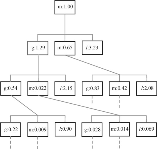
As an illustration the figure 1 shows a scheme of a number of layers in such a production process. The end product is located at the top of the pyramid (in this case a quantity of 1 ton of metal). Each lower layer represents the production factors, which are needed for the production in the layer above. The dotted lines are vertical production columns, which have been left out. The scheme is taken from the example, which will be discussed at the end of this column⁸.

The total quantity of labour, which must be expended for the generation of the product, can be calculated simply by means of the row vector v = a · B. The components of the vector are v_j = Σ_i=1ⁿ a_i × β_ij. It has been stated previously, that β_ij represents the required quantity of the means of production i for a unit of end product j. The multiplication with a_i transforms the physical quantity of i into the quantity of labour, which is expended in order to generate the quantity of j. In other words, the components v_j are the quantities of labour, which are required in order to generate a unit of the end product j.

The components of v are called the vertically integrated labour coefficients. The term vertical expresses, that they are the sum of all labour, which must be expended in that vertical production chain. The sum contains both the indirect labour, which was required to generate the means of production, and the direct labour. In the figure 1 all the bits of labour are indicated in the blocks with l in them. Since labour itself is not produced, the labour block does not have its own column.

The vector v is implicit in the formulas 2 and 3. For the combination of both formulas yields the formula v · y = L. Now note that y/L is simply the real wage w_R per unit of labour, at least in the case that the factor labour receives everything, which it has generated as end products. That is to say, w_R is the physical wage per unit of labour. Apparently that wage satisfies v · w_R = 1. In this situation a unit of labour is paid exactly that, which it has produced, namely 1.

The reader may feel, that the preceding arguments are too abstract. Therefore, in the following paragraph an example is presented, in order to make the matter more appealing and transparent. Anyway, the practical application of the previous formulas cause several problems. In the Leninist books about the planned economy much effort is invested in the analysis of the technical coefficients. For instance, studies are made of the changes in the end resuls, when a coefficient is adjusted⁹.

Decomposition of the price in dated quantities of labour

In this paragraph the dating in the price system of the production process is studied. Since a year ago the first column about price setting appeared, several columns have elaborated in detail on this theme. For the sake of convenience, the arguments are repeated here, and several insights from the former Leninist states are added. The price formula in its most general form is

(5)     p_j × Q_j = Σ_i=1ⁿ (p_i × q_ij) + D_j

In the formula 5 the dependence on time is ignored, for instance in the case of economic growth. The quantity p_i represents the price of the product i, and D_j is the added value in the branch j ¹⁰.

The added value supplies the income in order to pay the wages, and to accumulate funds for future investments. Also taxes must be remitted to the state, so that the necessary infrastructure can be maintained at the desired level. In principle the formulas 1 and 5 imply, that the summed added values must satisfy the relation Σ_j=1ⁿ D_j = Σ_i=1ⁿ p_i·y_i. In other words, the total "income" must equal the value of the total end product¹¹.

However, the reality is different. Both in the planned economy and in the private market economy the price formation of products is a subjective process, which is hardly amenable for a logical analysis. In the planned economy the prices are determined or steered at the central level, so that at least some systematics can be introduced¹². This process of price fixing by means of planned value modification has been described in a general manner by a previous column. In particular, it is common to modify the consumer prices (or prices for the final consumption) with regard to the prices for the means of production (the industrial or (in German) Erzeuger prices).

Such a differentiated price system is perhaps unavoidable in practice, but it is hardly accessible for a scientific analysis. And the plan also somewhat differentiated the efficiency r of the invested capital, in accordance with the social interests, that were attached to certain economic activities. Therefore, the central plan usually employs physical intertwined balances, whereas the value balances are merely derived and dependent on the physical ones. The price system was kept constant during the currency of the multi-year plan, because price fluctuations disturb the production.

These are the reasons that the Leninist economists (rightly so or not) have never paid attention to the integral price model. Therefore, in the present paragraph your columnist draws mainly from the neoricardian theory of Sraffa. In that model, which is based on perfect competition, the producer j receives in exchange for his production a yield according to the formula

(6)     p_j × Q_j = (1 + r) × Σ_i=1ⁿ (p_i × q_ij) + w × l_j

In the formula 6 w is the wage level. The efficiency r of capital can be interpreted as the profit rate, corresponding to the prevalent social conditions.

The interest must be paid from the profit. When it is supposed that the producers themselves receive an insignificant surplus, then r equals the interest rate. Apparently, together with the efficiency r there are n+2 unknown variables. The calculation of these variables becomes more transparent, when the quantities are removed from the formula 6. The division of the left- and right-hand side by Q_j yields

(7)     p_j = (1 + r) × Σ_i=1ⁿ (p_i × a_ij) + w × a_j

The producer j can not solve the formula 7 by himself. The prices for his raw materials and equipment are dictated by the market. The solution is only possible at the macro-economic level, where the formula 7 has the form of a vector:

(8)     p = (1 + r) × p · A + w × a

The solution is obviously¹³

(9)     p = w × a · (I − (1 + r) × A)^-1

If desired, the wage level can be taken as the numéraire. In that case the prices become relative, namely p/w.

The argument of the formula 4 can be repeated for the price formula 9, in order to make also a decomposition of the price:

(10)     p / w = a + a · (1 + r) × A + (1 + r)² × A² + a · (1 + r)³ × A³ + ...

The formula 10 can be explained in the same way as the formula 4. The price of a product unit must contain at least the wage sum of the labour, which is expended directly for its generation. That is the first term a·I in the power series. The second term represents the labour, which has been expended in the generation of the used means of production. This is called indirect labour, because it has been done during the previous period Δt. In the same way all following terms can be explained.

The difference with respect to the formula 4 is the term (1+r)ⁿ. It takes into account, that capital must yield a revenue. Consider for instance the second term a·A. It has just been stated, that it represents the labour, which has been expended in the previous period Δt. The investor wants to realize an efficiency r on the advanced wage sum, so that in the sale of the end products a·A must be "taxed" with a markup r. The subsequent terms in the power series correspond to even earlier periods, so that a markup is put on the markup¹⁴.

The formula 10 shows that the price is composed of contribitions from the direct and indirect labour. Whereas in the formula 4 all layers of production are treated equally, they are clearly dated in the price formula 10. One recognizes in this formula also the complex manner, in which fluctuations of the wage level and of the efficiency influence the prices. For the wages and the efficiency must both be paid from the value of the end product p·y. For instance in case of a falling wage level w room will be created for an increase of the efficiency r. Each term in the power series will show a different response¹⁵.

An example of the decomposition and dating

Certainly for the present theme an example will serve to enliven the theory. Again the familiar example of an economy with two branches (n=2) is employed, namely the agriculture (branch 1) and the industry (branch 2). In the agriculture 20 workers (20 units of labour, l_g = 20) produce 12 bales of corn (Q_g = 12) during a production period. In the industry 10 workers (10 units of labour, l_m = 10) produce 3.1 tons of metal (Q_m = 3.1) during the same production period. The nett or end product is y = [3, 0.9].

The production technique is fixed by the technical coefficients. The values of those coefficients a_ij and a_j are displayed in the table 1. If desired the reader can check for himself, that the formulas 1 and 2 are satisfied. The reader is reminded once more, that the values represent the direct use of quantities per unit of product during its generation.

Next the coefficients β_ij of the total input have been calculated, which together form the matrix B of the formula 3. They express the quantities of means of production, which are needed in total per unit of end product. Their value is the sum of the direct and indirect input. Also the components of the vector v of the vertically integrared labour have been computed. All those values are also included in the table 1. The reader may remember, that the value of the direct input is normalized with respect to the total product, whereas the value of the total (full) input is normalized with respect to the end product¹⁶.

For instance in the agriculture 0.4167 bales of corn are needed as a direct means of production in order to generate a single bale of corn in the total product. However, in total 1.913 bales of corn are needed in order to generate that single bale of corn in the end product. Apparently the first branch requires an input of 0.913 bales of corn and 0.08989 tons of metal during the production process of one bale of corn for the end product.

In the same way the industry requires 0.6452 tons of metal as a direct means of production for the generation of a single ton of metal. However, in total 3.145 tons of metal are needed for the generation of that single ton of metal. Apparently, the second branch requires an input of 6.956 bales of corn and 2.145 tons of metal during the production process of one ton of metal for the end product.

Consider again the end product y = [3, 0.9], then the agriculture requires an input of 2.739 bales of corn and 0.2697 tons of metal in the production. The industry requires an input of 6.260 bales of corn and 1.931 tons of metal in the production. In total at the beginning of the next production cycle 9 bales of corn and 2.2 tons of metal are available as means of production¹⁷. This is of course also clear from the data in the first sub-paragraph of the present paragraph, when one calculates Q − y.

The formulas 3 and 4 show that the matrix B can be rewritten as a power series of the matrix A. The figure 2 shows the form of this decomposition for the present example¹⁸. The first term in the power series corresponds to the quantities, that are needed in the end product, and the second term represents the means of production, that generate this end product. The third term represents the generation of the means of production themselves, etcetera.

Figure 2: Decomposition of B in power series of A

In the preceding text the figure 1 has already been presented, which is an elaboration of the decomposition in the figure 2. The scheme in the figure 1 is restricted to the branch of industry, and thus concerns the second column in the matrices of the figure 2. The top of the pyramid corresponds to the unity matrix I. Here a ton of metal is located. The production factors, which have been consumed for its production, are shown in the layer below (g = corn, m = metal, l = labour). This layer corresponds to the matrix A.

In the same way the third layer corresponds to the matrix A². This becomes clear, when all quantities of the production factors in the scheme are added. The result is 0.54 + 0.83 = 1.37 bales of corn, and 0.022 + 0.42 = 0.44 tons of metal. This equals (apart from rounding errors) the second column of A². The fourth layer in the scheme is not completely displayed, but the reader will understand that it corresponds to A³. Etcetera.

Now consider the price system. The formula 10 shows that the price of a unit of product can be calculated from a power series of (1+r)×A. Incidentally, this expansion in a power series is only possible, as long as the efficiency r is small. In the present example the upper boundary of r is 0.395. A special case is r=0, because then p/w equals v. Then the price is clearly composed of a series of labour values. The first term is the direct labour input, and all subsequent terms represent the indirect labour, which is stored in the means of production.

In the general case with r≠0 the indirect inputs of labour are dated, and the simple summation of labour values is no longer valid. That is to say, in the general case the internal time structure of labour during the complete production process affects the prices¹⁹. As an illustration the formula 11 describes the form of p_g/w:

(11)     p_g/w = 1.667 + 0.7484 × (1 + r) + 0.3824 × (1 + r)² + 0.2210 × (1 + r)³ + ...

The normalized price rises for an increasing r ²⁰.

1. See Vorlesungen zur Theorie der Reproduktion (1988, Metropolis-Verlag) by L.L. Pasinetti. The book appeared in the Italian language in 1975. In 1977 an English translation Lectures in the theory of production was published. Your columnist likes to read in the German language; it is almost a Dutch dialect. Besides, the German editions are often cheap. (back)
2. The Dutch poet Jef Last had confidence in planned economies. His belief was strenghtened by the persistent economic depression in the Netherlands. In Twee werelden he writes: From steel, concrete and stones it grows / from human hearts and steel human will / from enthousiasm of the shock-troops / from science, from labour steady and still / and clearly flutters, above their strong deeds / the red flag from every tower spire. (back)
3. On p.102 of Volkswirtschafsplanung (1971, Verlag Die Wirtschaft) the East-German economists L. Reyher and P. Rohrberg call this formula the first fundamental equation of the intertwined model. This book has been acquired from the full cellars of the Berlin second-hand book shop Helle Panke. (back)
4. An extensive discussion about the material input in all spheres of economic life (production and circulation) can be found in the excellent book Volkswirtschaftlicher Reproduktionsprozeß und dynamische Modelle (1973, Verlag Die Wirtschaft) by the East-German economist Eva Müller. Also this book is bought from Helle Panke. It turned out that the daily practice of economic planning benefited from the availability of a large variety of different coefficients. One example from this large collection: the distribution or material part coefficient is defined as a^*_ij = q_ij / Q_i. See p.55 in the book, just mentioned. In Ökonomisch mathematische Methoden und Modelle (1965, Verlag Die Wirtschaft) by the well-known Russian economist V.S. Nemchinov (in the German language: W.S. Nemtschinow) a^*_ij is called the coefficient of the production output. See p.177 there. The book originates from a second-hand book shop in Leipzig. (back)
5. Eva Müller rightly argues on p.56 and further in Volkswirtschaftlicher Reproduktionsprozeß und dynamische Modelle, that actually the coefficients of the full material input should be given by the matrix B − I. For it is not logical to include the end product in the full input. However the habit turns out to be stronger than logic. For all other economists, including the Russian ones, identify the coefficients of the full material input simply with the elements of the matrix B.
   There is evidently no compelling reason to assume that the β_ij are constants, apart from the love of ease. For instance, on p.82 and further in Verflechtungs-bilanzierung (1975, Verlag Die Wirtschaft) by V.V. Kossov (in the German language W.W. Kossow; again acquired at Helle Panke) the alternative form Q_i = Φ_i(y) is proposed. In other words, the total quantities have the form of a vector function Φ, with as her arguments y₁, ..., y_n. In this more general case the branches are intertwined in such a way, that the expression ∂Q_i/∂y_j can herself be a variable function of y. (back)
6. See p.88 of Vorlesungen zur Theorie der Reproduktion. This expansion into a power series is well-known in the common mathematical analysis, where for a real variable x on has 1 / (1 − x) = Σ_n=0^N
xⁿ. Also on p.57 of Volkswirtschaftlicher Reproduktionsprozeß und dynamische Modelle (and other East-European books) an explanation is given with regard to the decomposition into a power series, but not nearly as detailed as in the book of the skilled educationalist Pasinetti. The decomposition is not only meaningfull fot the theory, but she is also convenient for computations. In many cases B can be calculated faster with the help of the power series than by an inversion of the matrix (I − A). (back)
7. Note that the series can be broken off after the (k+1)-th term, if desired. Then the remainder y_R is Σ_n=k+1^∞ Aⁿ·y. Now a kind of decomposition of Q has been created, where the static situation has been furnished with an artificial prehistory, Namely, suppose that at the time t=0 the society disposes of resources with a size of y_R. Those can be used in the production cycle of a duration Δt, where they must be reproduced themselves, and in addition an extra quantity A^-1·y_R. That is to say, the total product has grown. This growth process can be continued, where in each cycle the total product is used for the means of production. After k of those production cycles, so at the time t=k×Δt, the growth has advanced to such an extent, that a quantity A·Q of the means of production is available. Henceforth, the static production situation can be entered, where eternally a quantity Q is produced, and each time an end product y is removed from the circulation. Apparently this "trick" has constructed a possible growth path towards the static situation. (back)
8. The idea of the scheme can for instance be found on p.58 of Volkswirtschaftlicher Reproduktionsprozeß und dynamische Modelle and on p.68 of Ökonomisch mathematische Methoden und Modelle. Those schemes differ from the figure 1 in so far as Eva Müller and V.S. Nemchinov have chosen schemes, which end and thus have a deepest layer. On the other hand, the scheme in the example of your columnist extends in perpetuity to ever deeper layers. (back)
9. See for instance p.65 and further in Volkswirtschaftlicher Reproduktionsprozeß und dynamische Modelle, or also p.97 and further in Verflechtungs-bilanzierung. Such studies contribute little to the fundamental comprehension, and are mainly useful and interesting for veritable economic applications. (back)
10. See for instance p.102 in Verflechtungs-bilanzierung or p.210 in Ökonomisch mathematische Methoden und Modelle. Strictly speaking the deprecations must be included in D_j. But these are not really relevant for the fundamental comprehension. (back)
11. Namely, the formula 1 is Q_i = Σ_j=1ⁿ q_ij + y_i. Multiply this formula by p_i and sum over i. Sum the formula 5 over j, and combine both results. They can only both be true, as long as the equality holds, that is mentioned in the main text. (back)
12. Henriëtte Roland Holst - van der Schalk had confidence in planning. Therefore, in Heldensage she writes: This time the human genesis disengaged a / new force: the power of prospect, of / regulating conscience. / Like a sea of fire rages / and roars, roared and raged the fire of desire / downwards. But upwards the ideas are awake; / they weigh the pros and cons and know. Their cool splendor and / that wild roar forged the strong band / of a single will. The blind passion got eyes, / the reasonable insight got material power: / new, strong, magnificent rithms moved / the hearts. Truth conquered lies, / bloody dawn pushed back the night. (back)
13. When no efficiency of capital is realized (r=0), then the formula 8 obtains the simple form p = w × v. In that situation the costs can be attributed completely to the expended labour. (back)
14. Perhaps the reader is familiar with such calculations in the estimates of capital. There the flows of money are converted into their present value. For instance, suppose that during a series of n future periods a yearly income R(t) can be collected. Then the net present value) is NPV = Σ_t=1ⁿ R(t) / (1+r)^t. See p.504 and further in Managerial economics (1992, Macmillan Publishing Company) by P. Keat and P. Young. In the formula 9 the powers are in the numerator, because the investment has been done in the past, and the investors want to be compensated in the present for the loss of value. (back)
15. A falling wage level will naturally push up the normalized price p/w. But the effect of this rise has an uneven distribution in the power terms of the series, due to the term (1+r)ⁿ. The economist P.A. Samuelson, on p.631 and further in his classic work Handboek economie (1978, Aula-reeks, Het Spectrum), uses the power series to explain the switching between the various available production methods. Your columnist prefers the explanation by means of the wage-profit curve. The Dutch economist W. van Drimmelen discusses on p.190 and further in Meerwaarde en winst (1976, Socialistische Uitgeverij Nijmegen) the dating in a historical context, with references to Marx and von Bortkiewicz. He uses the decomposition to illustrate the transformation problem of the price theory of Marx. This approach aims to explain the properties of the marxist labour theory of value, but it results in rather cumbersome arguments. (back)
16. It is interseting to observe that the values of the vertically integrated labour coefficients v are exactly identical with the labour values of a bale of corn and a ton of metal, that have been computed in a previous column. See also further on in the text. (back)
17. Pasinetti performs a similar calculation on p.87 of Vorlesungen zur Theorie der Reproduktion. (back)
18. Pasinetti performs a similar calculation on p.89 of Vorlesungen zur Theorie der Reproduktion. (back)
19. See p.197 of Meerwaarde en winst. (back)
20. See also the figures in the column about the choice of the technique. (back)