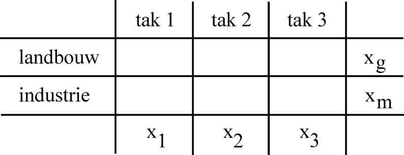
Figure 1: Classification of production in 3 branches
The book Volkswirtschaftlicher Reproduktionsprozeß und dynamische Modelle1 by the East-German economist Eva Müller is a source of inspiration for anybody, who is interested in dynamic growth. An earlier column describes the way in which she expresses two versions of the well-known national income model. In these models the national economy is presented as one large homogeneous sector. In two other columns it is explained how she calculates the economic growth at the level of the separate sectors or branches. The models of this type are founded on an input-output analysis and on an intertwined balance. It requires a detailed knowledge of the available production techniques. Müller considers two versions of the input-output analysis. The first variant yields an exact solution. The second variant is able to calculate the stock of capital goods, besides the total product. This additional information is paid by the necessity to revert to a numerical technique.
The so-called dynamic three-sector models are variants of the one-sector models. They have the additional merit with respect to their simpler ancestors, that they can calculate the total product. This implies that the development of the stock of capital goods (the fundamental fund) becomes visible, at least at the macro-economic level. The material flow in the system is revealed. Like the name indicates, this type of model is characterized by three (groups of aggregated) sectors or branches.
In the model of Biersack the national production is subdivided into the following three groups or branches2:
The figure 1 shows how the classification operates. Each type of production (for instance the agriculture, and the metal industry) is classified in either the branch 1, 2 or 3. Certain types of production make goods, that are applied in various manners (for instance: corn as a consumer good, and also as a material, such as biofuel). So such production must be divided across various branches. There is also production, where the product clearly belongs to one branch (for instance: a milling machine). After the completion of the classification of production, in each branch i the product volumes are summed (aggregated) into a single product xi (M, G of K)3.
The coefficient of the effectivity of the fundamental fund is defined as
(1) ki(t) = xi(t) / gi(t)
In the formula 1 xi is the production of the branch i. That is to say, xi equals M, G and K for respectively i = 1, 2 and 3. The quantity gi represents the stock of the fundamental fund in the branch i.
The material flows are determined by the matrix A, which has as its elements the coefficients of the material input in the three branches. Since all the material production is aggregated (combined) into the first branch, the matrix A takes on the form of the vector a(t) = (ai(t)). She satisfies the relation
(2) x1(t) = Σj=13 aj(t) × xj(t)
In the formula 2 Σ is, like always on the webportal, the mathematical symbol for summation.
Investments change the available stocks of the fundamental fund. They represent a change in time, which occurs during an interval Δt. On the one hand they are replacements, that substitute the worn equipment in the preceding period. The replacements in the branch 1 are wi(t) × gi(t-Δt), where wi(t) is called the rate of replacement. On the other hand they are the nett investments iN(t), that add new production capacity to the existing stock. For the i-th branch these are defined simply by Δgi(t) = gi(t) − gi(t-Δt). Together the replacements and the nett investments form the gross investments. The gross investments i(t) at the time t must be made already in the preceding period. Since all the production of the fundamental fund is aggregated in the second branch, i(t) = x2(t-Δt) holds. Thus it can be concluded, that one has:
(3) x2(t-Δt) = Σj=13 (wj(t) × gj(t-Δt) + Δgj(t))
In the dynamic three-sector models it is common to introduce the so-called steering-parameters, which express how the investments are allocated to the three branches. These so-called investment share coefficients are defined by
(4) ui(t) = Δgi(t) / iN(t)
Evidently one has u1 + u2 + u3 = 1, so that one of the steering parameters is fixed by the other two.
The steering parameters u(t) serve to optimize the performance of the economic system. A target function is chosen, and values for u(t) are identified, that yield the largest value of the target function. The performance of the economy is always measured by the consumptive supply. Therefore a logical target function is
(5) ZI(T) = x3(T) = K(T)
In the formula 5 T refers to the time, where the target function is evaluated. The disadvantage of the formula 5 is that the maxinal consumptive supply at the time T does not guarantee any consumptive supply at the other times. Therefore often the growth path is evaluated for a longer time period T×Δt, and then aims to optimize the target function ZII(T), defined by
(6) ZII(T) = Σt=1T x3(t)
Now the formulas 1, 2, 3 and 4 can be combined in the equation (just plain computation)
(7) Δgi(t) = ui(t) × (c1(t-Δt) × g1(t-Δt) + c2(t-Δt) × g2(t-Δt))
This is the fundamental formula for the dynamic three-sector model. In the formula 7 the quantities c1 and c2 are defined by
(8a) c1(t) = -w1(t+Δt) − w3(t+Δt) × (1−a1(t))×k1(t) / (a3(t)×k3(t))
(8b) c2(t) = k2(t) − w2(t+Δt) + w3(t+Δt) × a2(t)×k2(t) / (a3(t)×k3(t))
Suppose that the target functions ZI(T) or ZII(T) or yet another must be evaluated. Then it is desirable to determine in advance the range of possible values of the steering parameters in the formula 4. For their range of values is bounded. This can be shown easily for the case that both k and a are independent of time. Then x can be eliminated from the formula 2 by means of the formula 1, and the result can be substituted into Δg(t) = g(t) − g(t-Δt), so that one has
(9) k1 × Δg1(t) = Σj=13 aj × kj × Δgj(t)
The formula 4 can be used to replace Δgj(t) by uj(t). A simple elaboration of the resulting expressions leads to:
(10) u1(t) = (a3×k3 + u2(t) × (a2×k2 − a3×k3) ) / ((1−a1)×k1 + a3×k3)
Now u3(t) = 1 − u1(t) − u2(t) implies that one has
(11) u3(t) = ((1−a1)×k1 − u2(t) × ((1−a1)×k1 + a2×k2) ) / ((1−a1)×k1 + a3×k3)
Since all three investments share coefficients ui(t) must satisfy 0 ≤ ui(t) ≤ 1, the formulas 10 and 11 put limits to their range of values. In the following text this will be illustrated by means of an example.
The formula 7 can be solved in an exact way, if the time interval Δt is taken to be infinitesimally small. In mathematical terms this implies Δt → 0. Then one has Δgi(t) = ∂gi(t)/∂t × Δt, so that the formula 7 changes into
(12) ∂gi(t)/∂t = ui(t) × (c1(t) × g1(t) + c2(t) × g2(t))
In the preceding it has been argued, that the model becomes rather simple for the case of constant quantities a, k and w as a function of time. Then the formula 8a-b implies that also c1 and c2 must be constant. Assume in addition that u is independent of the time t. Then the formula 12 has a simple solutionon:
(13a) g1(t) = eα×t × u1 × γ / α + c2 × β / α
(13b) g2(t) = eα×t × u2 × γ / α − c1 × β / α
(13c) g3(t) = (eα×t − 1) × u3 × γ / α + g3(0)
The constants in the formulas 13a-c are defined by
(14a) α = u1 × c1 + u2 × c2
(14b) β = u2 × g1(0) − u1 × g2(0)
(14c) γ = c1 × g1(0) + c2 × g2(0)
An example may help to clarify the theory. In this calculation the numbers are copied from the economic system in an earlier column about the intertwined balance. Of course this choice is arbitrary. But recurring values of the quantities in the various models give a feeling of familiarity, and make it easier to identify their similarlties and differences.
In the column the economic system produces bales of corn in the agriculture and tons of metal in the industry. Both products can be employed in the three branches, namely material, equipment and consumption. Now the problem arises, that within a branch i the bales of corn and the tons of metal must be aggregated into a single production volume xi. See the figure 1. Besides in the formula 4 the investments Δgi can be combined into the aggregated nett investments iN. But evidently bales of corn and tons of metal can not possibly be brought under one denominator. Therefore in the calculation only the production in the agriculture (corn) will be considered. Then there is just one denominator or measure, namely corn. The reader sees how the comparison of the various columns and models stimulates reflection.
In the previous column at the time t=Δt it turns out that xg = 24.47 (bales of corn), (A x)g = 17.14, ig = 6.232, yg = 1.1 and Γg = 17.62. These numbers are taken here as the starting point on t=0. Thus a somewhat curious economic system exists, where corn is both the only material, and the only means of production, and the only consumer good. However that may be, this does not degrade the numbers. If they are transposed to the present model, the cited numbers lead to xg(0) = (17.14, 6.232, 1.1). This distribution can also be used to divide Γg, resulting in gg(0) = (12.45, 4.289, 0.88). The following parameters are taken to be constants for all branches and all times:
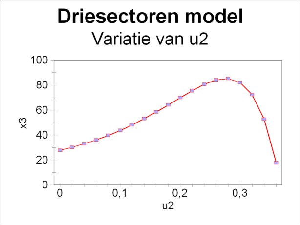
Figure 2: consumption x3 versus parameter u2
The formula 8a-b shows, that now also c1 and c2 are constants. One finds for them respectively the values -0.03347 and 1.456. Incidentally, in the infinitesimal case of Δt → 0 the solution for g is given by the formulas 13a-c. Before computing the solutions, first the collection {u} of allowed steering parameters must be determined, by means of the two linear relations 10 and 11. Substitution of the numbers in these formulas yields u1 = 0.5975 + 0.09703 × u2 and u3 = 0.4025 − 1.097 × u2. Therefore the allowed values of u2 lie in the range [0, 0.4025] and those of u2 lie in the range [0, 0.3669]. Thus the steering parameter u1 lies in the interval [0.5975, 0.6332] 4.
Now the problem of optimization is completed by means of the continuous solution, that is given in the formulas 13a-c. They can be obtained by a systematic variation of the steering parameter u2. Especially important is the consumptive supply x3(t) = 1.25 × g3(t), since it determines the prosperity of the society. In order to limit the amount of computations, the quantity ZI in the formula 5 is chosen as the target function, that must be optimized. The time period T, that is addressed by the optimization procedure, is set at T=10.
The results of the variational computation are shown in the figure 2. The target function ZI and thus also the consumptive supply x3(10) are maximal for u2=0.28. Then one has u1=0.62 and u3=0.10. The form of this curve reminds of a similar curve in the column about the one-sector models. There also the consumptive supply is studied, albeit in connection with the variation of the rate of accumulation. It is concluded, that in principle a larger accumulation raises the future expectations for the consumptive supply. However, this positive development is slowed down, when the accumulation becomes excessive. For then the investments seizes almost the entire national income. A similar development can be seen in the figure 2.
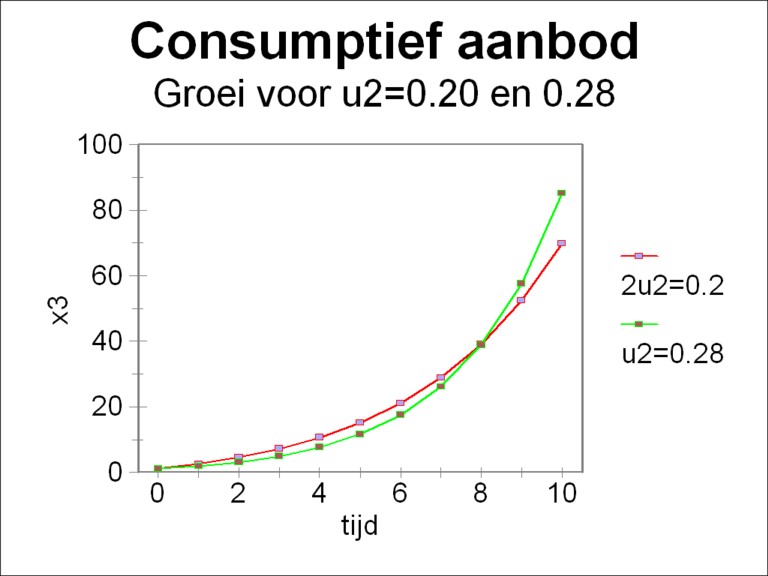
It is true that the figure 2 contains all necessary information, but she does not make immediately clear, why u2=0.28 yields a larger productive supply than for instance u2=0.20. For the sake of completeness the figure 3 shows the behaviour of x3(t), both for u2=0.20 and 0.28, within the time span T=10 5. The figure illustrates that the parameter u2=0.28 is definitely not superior to u2=0.20 for all times. Only at the time t=9 does the curve belonging to u2=0.28 surpass the curve of u2=0.20. If the target function would have been evaluated at a smaller T, for instance T=5, then u2=0.20 would be preferable above u2=0.28.
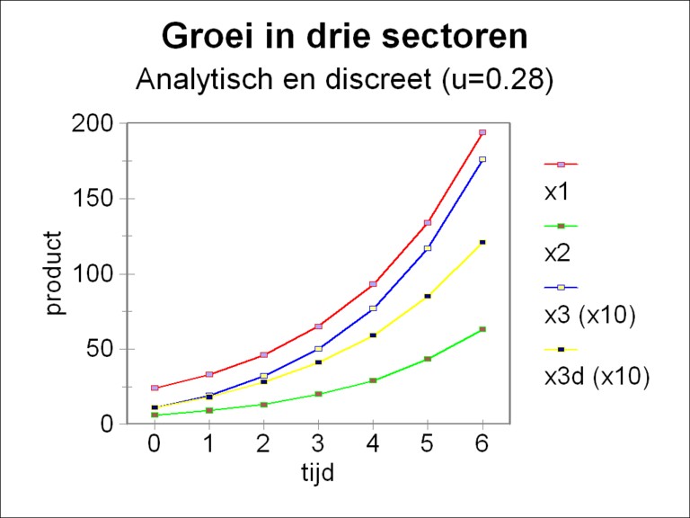
At the beginning of this column it has been stated that the real power of the three-sector models is their ability to calculate the development in time of the stocks of capital goods (the stock of the fundamental fund). An example of such simulations is shown in the figure 4. The formulas 13a-c have been used with the same numbers as before in order to compute x1(t), x2(t) and x3(t), for six timesteps. Here the volume of investment is split by means of the steering parameter u2 = 0.28, which is the optimum, that has been found just now. The production in the third branch is scaled up with a factor of 10, in order to show all curves clearly within a single figure. Here the factor α of the formula 14a has a value of 0.387. Apparently the rate of growth of the economic system equals 38.7%.
Unfortunately in most cases the differential equation 12 will not be solvable in an analytic manner. Then the solution must be computed with a numerical method, such as the formula 7. Therefore it is interesting to investigate deviations of the numerical solution due to numerical errors. That can be done by a comparison of the numerical solution with the analytical (exact) solution, at least so far as possible. Such a comparison is shown in the figure 4, where also the discrete solution x3 is shown, computed with the formula 7 (x3,d, scaled up with a factor of 10).
The figure illustrates that at first the results of the two methods of solution for x3 almost coincide. But after the third time step they start to separate, and for T=10 (not shown) the analytic solution is already more than 80% larger than the numerical one. The cause of this kind of deviations has already been discussed in an earlier column. Namely, in the numerical approach with the formula 7 at the time t the quantity of capital goods Δgi, that has been made in the preceding period [t-Δt, t], is added at one go. However, in reality the stocks gi increase in a continuous manner. So their estimate with the terms gi(t-Δt) in the formula 7 is too low.
Eva Müller points out in her book, that the formula 7 does represent the reality in a situation, where the newly made capital goods (equipment) are employed with a certain delay (Δt) 6.