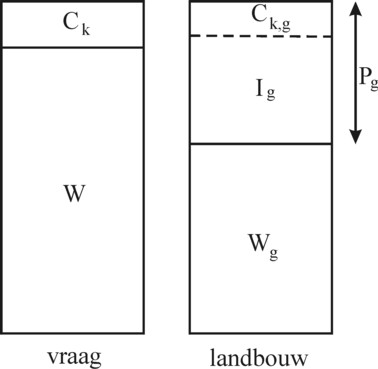
Figure 1: Income distribution
An important question in the research of business cycles is how the market fluctuations, which are naturally inevitable in an imperfect world, are maintained by the economic system itself. In a previous column about the theory of Kalecki it has already been remarked, that indeed the system can under certain circumstances bring itself in a state of oscillation. The present column illustrates this phenomenon by means of an example, which originates from the well-known economists Joan Robinson and John Eatwell. It is a two-sector model.
The example can be found in the popular introductory textbook Inleiding tot de moderne economie1. It concerns an application of the theory of business cycles according to Michal Kalecki. The example does not add new knowledge, but it does illustrate what the practical consequences are. In particular for the given situation it is shown, that the theory indeed predicts an economic crisis. The assumption of two branches is not typical for the theory of Kalecki, but she does not change the arguments in a significant way. She is especially interesting, since it becomes apparent how in each branch the crisis develops in a different way. Incidentally, the example in the present column uses different numbers than those of Robinson and Eatwell.
Just like the many preceding columns the present example assumes, that the economic system consists of two branches: the agriculture and the industry. The agriculture produces corn (with the bale as its unit) and the industry generates metal (with the ton as the unit of weight). The agriculture disposes of lg=20 units of labour time (for instance 20 man years), which produce nett Qg,N=1.8 bales of corn. The industry disposes of lm=10 units of labour time. For the moment the system is in a static situation.
| agriculture | industry | nett product | |
|---|---|---|---|
| corn | qgg | qgm=0 | Qg,N=1.8 |
| metal | qmg | qmm | Qm,N=0 |
| workers | lg=20 | lm=10 | |
| production | Qg | Qm |
The agriculture uses qgg bales of corn as seeds for sowing, and qmg tons of metal for tools, which together form her means of production. The metal is obviously supplied by the industry, in such quantities that the worn-out tools can be just replaced. The industry itself employs merely qmm tons of metal for her means of production, and these tools are produced in her own branch. The table 1 presents the system in the form of a matrix. The rows describe the distribution of the gross product over the branches. The columns describe the production technique of the concerned branch.
The investments Ig of the agriculture require payments to the industry, whereas the investments of the industry are done in her own branch. Note, that this concerns gross investments. The metal is merely replaced, but not extra expanded. The nett investments are zero. In a mathematical form the exchange between the two branches becomes
(1) Ig = Wm + Pm
Here Wm and Pm are respectively the wage sum and the profit sum in the industry. The formula 1 has been derived first by Karl Marx2. She must be immediately elucidated, because in the approach of Robinson and Eatwell the depreciations and the replacements are included in the profit - contrary to the idea of Marx. In the following this aspect will be mentioned again, sometimes in the footnotes. The investment Ig on the left-hand side is a productive demand, which is satisfied by means of the surplus product qmg = Qm − qmm of the industry. The right-hand side describes the costs, which are made by the industry, and the markup for profit as well3.
For the economic system as a whole the income is designated by the symbol Y (without index), just like in the previous column about Kalecki's theory of the business cycles. That is to say, for a given total wage sum W and profit sum P the definition of Y is
(2) Y = W + P
Since the depreciations are included in the profit P, here Y is the so-called gross added value. The economic system chooses to use corn as its only legal currency. Income consists by definition of corn. Then the nett product Qm,N of the industry is naturally zero. The wage level is 0.05 bales of corn per unit of labour, so that the wage sums in the agriculture and in the industry are respectively Wg=1 and Wm=0.5 bales of corn.
As usual the profit Pi of branch i (i=p or m) must conform to the general profit rate r of the system. However, the definition of the profit rate differs somewhat from the usual approach, for she is r = P/W. That is to say, the profit Pi is related to the wage sum in the branch, in the form r×Wi. It is evident that both the agriculture and the industry dispose of metal tools, but these capital goods do not yield any rent. They are merely present in the total product, and not in the nett product4. It has already been mentioned, that they do exert influence, by means of the replacements.
After fixing the productive sphere of the system in this manner, now the consumption must be modelled. The society has two classes, one for the factor labour and the other for the factor capital. The class of the capitalists is formed by the entrepreneurs themselves. The factor labour expends his complete income on food and other household ware (workers spend what they earn)5. Since there is no permanent staff, all labour is productive. Therefore the wage sum is proportional to the gross added value Yi in the branch (i=g or m), where the constant of proportionality equals the labour productivity api = Yi / li.
The consumption function of the capital owners is
(3) Ck(t) = Ca + ck × P(t-θ)
In the formula 3 Ca is the autonomous consumption, which in this example is put equal to zero. The marginal consumption quote ck is put equal to 0.25, and the time lag θ equals a unit of labour time (for instance a year). The lag expresses the delayed adaptation of the consumption pattern of the capitalist to changes in their income (the profit of the concerned branch). In the present situation, which for the moment is static, the profit does not vary with time.
In the previous column it has been stated that capitalists earn what they spend. Their profit is determined by the amount of investments. The application of the formula 6 in that column, together with the insertion of Ca=0, leads to
(4) P = I / (1 − ck)
That is to say, the entrepreneurs invest 75% of their profit. Now the profit rate r can be computed first, and next the seize of the total income Y. The application of the formula 1 leads immediately to r=0.8, or 80%6.
The determination of Y raises the question how the investments Im of the industry in itself must be computed. This column follows the approach of Robinson and Eatwell in their book. Since that approach is rather cumbersome, and actually does little to increase the insight, your columnist refers for the explanation of their argument to a footnote7. There it is shown that one has Ym=0.9 (measured in bales of corn). The quantity Yg (the gross added value, or the total income of the branch) is conputed simply from Yg = (1+r) × Wg = 1.8 bales of corn. The table 2 summarizes all these numbers, and the figure 1 depicts the situation.
| agriculture | industry | total | |
|---|---|---|---|
| W | 1 | 0.5 | 1.5 |
| P | 0.8 | 0.4 | 1.2 |
| Y | 1.8 | 0.9 | 2.7 |
| I | 0.6 | 0.3 | 0.9 |
Some explanatory remarks with regard to the table 2 and the corresponding figure 1 are in place. First, it is obvious, that the table contains several double counts. A part of the profit sum Pg reappears in the industry in the shape of the wages Wm. But also the profit sum Pm creates extra employment in the industry. Within the industry, profit is converted into wages as well. This has been explained in the footnote. The double count is due to the absence of a time index in the static situation. In fact a part of the profit originates from the investment in wages during the previous time step θ 8.
The investment Ig is a demand for tools (metal), which represents a value of 0.6 bales of corn. Here the exchange relation of bales of corn and tons of metal is irrelevant. The same holds for the investment Im with a value of 0.3 bales of corn. Both investments are paid from the profit sum of the concerned branch. In the footnote it has been explained, that the investment Im (and thus also the profit Pm) contains a part with a value of 0.1 bales of corn, which is merely required for book-keeping, and which is not really expended.
It can be concluded from the preceding arguments, that the system is a collection of causal relations. They illustrate how investments influence among others the total income9. In each branch the profit sum has a size P=r×W. And the investments are I = (1 − ck) × P. Since according to the formula 2 the total income Y equals W+P, the investments equal Y × (1 − ck) × r / (1+r). In numbers this is Y = 3×I. This explains once more, now in a different manner, why, due to the sum 0.1 in the book-keeping of Im, the agriculture must not invest Ym, as suggested by the formula 1, but merely Ym − 0.3.
Next consider the following example. Let the economic system be static, but with investments Ig in the agriculture, which are 0.1 larger than in the table 2. How will these two situations differ (this implies a static comparison, not a transition from one situation to the other)? Then the economic structure dictates a larger profit in the agriculture, namely 0.1333. According to the formulas, just mentioned, the total income in the agriculture must be increased with 0.3 bales of corn. And the total income in the industry (the gross added value, including the term for book-keeping) rises by 0.15 bales of corn.
This increase is actually caused by the higher income of the industry, which creates an extra demand in the agriculture. The agriculture must produce more in order to satisfy the demand, but this creates once more an extra demand, namely those of her own extra employed labour and capital. Thanks to the expansion the profit is raised in such a way, that the agriculture can pay for the extra investments (capitalists earn what they spend!).
The previous paragraph may give food for thought, yet it is actually only presented as an introduction for the calculation of the conjuncture in the system with two branches. The approach in the model of Robinson and Eatwell is again used, albeit with adapted numbers10. Here all aspects of Kalecki's theory of business cycles become visible. First, this requires the assumption, that the agriculture and the industry dispose of a certain reserve in their production capacity. In other words, the utilization of the production factors (including the factor labour) is less than 100%. In a situation, where labour is added, idle tools must naturally be available for that extra labour.
The approach of Robinson and Eatwell models the system by computing all quantities by means of discrete time steps θ. The size of θ can be chosen at will, for instance a man year of labour. Since θ appears in the formula 3, the consumption of the entrepreneurs has a lag of exactly one time step. Contrary to the situation of the previous paragraph, here θ influences the level of consumption during the business cycle.
Robinson and Eatwell choose for the agriculture an investment function of the shape, which has been proposed by Kalecki (see the formula 8 in the previous column). Her formula is
(5) Ig(t) = Ig(t-θ) − 0.0565 + 0.5 × ΔPg(t-θ)
The reduction by 0.0565 implies that the entrepreneurs in the agriculture are somewhat more reluctant than in the previous paragraph, and they reduce their investments even for the case of a steady profit Pg 11. According to the formula 5 the entrepreneurs in the agriculture are willing to expand and do nett investments, when the rise of the profit is appreciable. Also here the lag in the behaviour is exactly one time step large.
The calculation of the business cycle starts with the situation in the table 2. The entrepreneurs in the industry invest still their total profit, as far as they do not consume it themselves. In the initial situation (t=0) one has Ig(0) = Ig,a. That is to say, they consist of the autonomous investments, which are just sufficient for the replacement of the worn-out tools. At the time t=0 an external "disturbance" occurs. Namely, the entrepreneurs in the agriculture for once take up a credit at a bank, because they want to do a nett investment. They place an extra order with the industry for tools. In order to execute the order the industry must hire 5 extra units of labour. Then the production capacity of the industry is completely utilized.
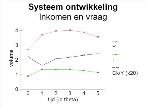
The utilization of the branches is an essential aspect in the study of business cycles. Kalecki points out, that after a full utilization of the capacity the economy can not grow further, at least for the moment12. She has reached her ceiling. So in the example this phenomenon occurs in the industry. From that moment onwards the development of the system will be followed step-by-step, in intervals with a duration of θ. The computation herself is wisely moved to a footnote13. The findings are presented in the table 3. Moreover, the figures 2 and 3 display the developments in respectively the separate branches and the economic system as a whole.
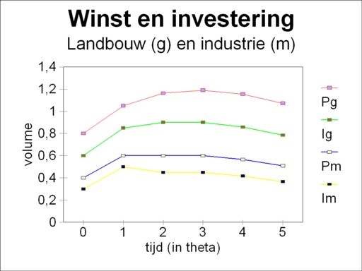
| agriculture | industry | |||||||
|---|---|---|---|---|---|---|---|---|
| t/θ | Wg | Pg | Ck,g | Ig | Wm | Pm | Ck,m | Im |
| 0 | 1 | 0.8 | 0.2 | 0.6 | 0.5 | 0.4 | 0.1 | 0.3 |
| 1 | 1.313 | 1.05 | 0.2 | 0.85 | 0.75 | 0.6 | 0.1 | 0.5 |
| 2 | 1.453 | 1.163 | 0.263 | 0.9 | 0.75 | 0.6 | 0.15 | 0.45 |
| 3 | 1.488 | 1.191 | 0.291 | 0.9 | 0.75 | 0.6 | 0.15 | 0.45 |
| 4 | 1.445 | 1.156 | 0.298 | 0.858 | 0.708 | 0.566 | 0.15 | 0.416 |
| 5 | 1.341 | 1.073 | 0.289 | 0.784 | 0.639 | 0.511 | 0.145 | 0.366 |
In the first row (t=0) the numbers from the table 2 reappear. In both branches the wage- and profit-sum maintain a ratio of 1/r = 1.25. In the second row (t=θ) the extra investment ΔIg = 5 × 0.05, which results form the order by the agriculture, affects the profit sum Pg, and in the industry it affects the wage sum Wm. For the following rows the calculation is straightforward. First, for each t=n×θ the change of the profit ΔPg((n-1) × θ) is computed. Next Ig(t) is computed from the investment function (formula 5).
The change of the profit at (n-1)×θ yields also the change of the consumption ΔCk,g(t) of the entrepreneurs in the agriculture. There the change of profit is ΔPg(t) = ΔCk,g(t) + ΔIg(t). And ΔWg(t) is 1.25 times as large. Furthermore the change of the profit ΔPm((n-1) × θ) yields the change of the consumption ΔCk,m(t) of the entrepreneurs in the industry. Next there the wage sum can be computed from ΔIg(t) = ΔWm(t) + ΔCk,m(t). Then the profit Pm(t) and the investment Im(t) are also known.
The reader will perhaps believe, that the fall continues after t=5×θ. Actually, with this investment function the fall will never stop. But the point has been made, namely that due to the structure of the economic system a crisis can occur by itself, without exogenous causes. And that was the whole purpose of the effort. The figure 3 shows that even a constant investment can already lead the system in a crisis. The quantity Ck/Y illustrates that in the recovery phase the entrepreneurs are less inclined to consume14. In the fall the consumptive behaviour has a lag, so that the consumptive demand improves, at least in a relative manner. This anti-cyclical behaviour underlies the under-consumption theories.
Several concluding remarks must be made. The implicit assumption is, that the agriculture will not hit the ceiling. As soon as the order at the time t=0 has been completed, the production capacity in the agriculture will be larger than before. It has not been stated, when those extra tools will be delivered. For that is not very relevant. And the question can be raised, whether the example is useful. Robinson and Eatwell believe it does. It may indeed help to see how the crisis develops.