
Figure 1: graphic arts
Herbert Sandberg
The present column shows, that the intertwined balance in kind can be transformed into a value balance. It is obvious, that this first requires a price formation. The presented theories are copied from the books Ökonomisch-mathematische Methoden und Modelle by V.S. Nemchinov, Verflechtungs-bilanzierung by V.V. Kossov, and Volkswirtschafts-planung by an East-German collective of authors1. The last two mentioned books originate from the second-hand bookshop Helle Panke in Berlin. An important aspect is the aggregation of product groups and of branch groups.
On this webportal the intertwined balance is a popular theme. It was first addressed two years ago, in the column about the fundamental model of the dynamic balance. Then the variables are still expressed in kind, that is to say, in physical units. Consider an economic system, where N products are traded. The starting point of the model is the formula
(1) x = A · x + y
In the formula 1 x represents the total social product. It is a vector with components xi, which represent the quantities of the product i (with i = 1, ..., N). The dimension of the vector is N×1, so that he has the form of a column. The vector y represents the nett product, which remains after the completion of the production process. For, a part of the production x is needed as a raw material, semi-manufactured article, or equipment. The part of x, that is reserved for the production, is represented by A·x. Here A represents the matrix with elements aij = xij / xj. The variable xij is the quantity of product i, which is needed for the production of a quantity xj of product j. Therefore A is a square N×N matrix. The aij are called the production coefficients, or in the Leninist terminology the coefficients of the direct material use.
The production technique is fixed by the matrix A, and is naturally determined by the social level of knowledge2. In that manner the formula 1 could represent the operation of all separate enterprises. In practice that makes no sense, and it is tried to categorize the enterprises in branch groups. However, two enterprises are never completely identical, nor are their products. Therefore each choice of categorizing (also called aggregation) is subjective. The most obvious choice is the formation of product groups. However, there are so many of these, that in general a further aggregation is inevitable. Then units of differing products are added, and that is only possible by means of their value or piece price. A need for a price system arises3.
Once this portal discussed the price system as a theme, even before the intertwined balance, namely in the column about the neoricardian theory. It is true that this theory is elegant, but she makes two rather restricting assumptions. First, she performs calculations with a uniform profit rate for all branches. And second, she ignores that a single product can have different prices, depending on its application. The analysis with intertwined balances does not need these assumptions. Besides the balance in kind, the material balance and the value balance are used4.
In the calculations with the material intertwined balance it is assumed that each product i has a unique price pi. Then the quantity xi has a value pi×xi. The coefficients of the material balance are expressed in value, and can be calculated from the balance in kind with the formula aijM = aij × pi / pj. The corresponding matrix formula is simply5
(2) AM = P · A · P-1
In the formula 2, P is the diagonal matrix with on the diagonal the values pi. That is to say, pij = pi × δij, where δij is the Kronecker delta, known from mathematics. The matrix P-1 is the inverse matrix of P. The formula 2 shows in a straightforward manner that the change of the price of a single product affects the change in value of the other products.
The construction of the value intertwined balance is based on the other extreme, namely the hypothesis that the price of each product i depends on its application j. In other words, when an entrepreneur makes a product j, and in it uses the product i as a raw material or semi-manufactured article, then he pays for the product i a piece price pij. The coefficients of the value balance are also expressed as values, and can be calculated from the balance in kind with the formula aijW = aij × pij / ρj. In this formula ρj is the average piece price, which is paid for the product xj.
Since the costs of production always remain the primary basis for the piece price, in practice the price will not depend very much on the application. Yet different prices occur, as has already been explained in the column about the Russian planned economy. For instance, an additional cost is caused by the transport of the product to the end user. That even leads to separate territorial price zones. And the sales tax (say VAT) can differ, depending on the application of the product.
Differences in prices can also occur in the invoices within enterprises. Sometimes the enterprise uses a part of its own production, charging another price in this operation than the market price. This is called the sales within the enterprise. In fact this invoice distorts the real costs, so that nowadays it is has fallen somewhat in disuse. All these price differentiations moderate the practical importance of the neoricardian theory with its unique price.
The column about planned prices distinguishes between the industry price pi of a given product i and its consumer price πi. It follows that the total product xi has an average "gross" piece price of ρi, where one has pi ≤ ρi ≤ πi. Thanks to these prices the formula 1 can be rewritten as a value balance (also called the summarized material balance)6
(3) ρi × xi = pi × Σj=1N aij × xj + πi × yi
The formula 3 separates the total product ρi×xi in the industrial markets and the consumer market of end products. However, the same total product can also be separated according to the costs, which must be made for its production
(4) ρi × xi = Σj=1N pj × aji × xi + Σj=1N wj × fji
Note, that in the formula 4 the matrix indices are exchanged in comparison with the formula 3. Thus Σj=1N pj × aji is the i-th component of the vector p·A. In the formula 4 fij is the quantity of the production factor i, which is needed in order to generate a quantity xj. The production factor can be labour, or capital, or land, or even the state or all other kinds of factors, which can possibly contribute to the profit of the enterprise. The reward of the production factor i has a value wi. Therefore Σj=1N wj × fji (the i-th component of the vector w·F) is the part of the national income, which is generated in the enterprise or the branch i.
An interesting result can be obtained by summing over i both the formula 3 and 4, and subsequently compare them. Namely, it turns out that
(5) Σi=1N πi × yi = Σi=1N Σj=1N wj × fji
Expressed in words the formula 5 states, that the value of the total nett product must equal the total national income. This striking identity has been mentioned already in previous columns, but the formula 5 explains the roles of the product prices and the factor incomes. For instance, when the wages are raised, then the nett product must also rise. If this does not happen, then the prices will rise, which causes inflation. Or one could lower at the same time, for instance, the interest or the taxes.
In the introduction it has been stated, that each entrepreneurial operation combines activities at the micro level. When for instance two branch establishments of an enterprise generate (almost) the same product i, then the two activities can be aggregated without problems. Then together they generate the product i with the average technique, weighed with the two sizes. Such an aggregation is impossible, when the two products are significantly different. In that case the products have a different value or product-price, and this must be taken into account during the aggregation.
Moreover it is conceivable, that the subject of interest is not a separate product group, but the sales of a branch group, which produces various products. An obvious example is the case of enterprises, which produce various products with identical production processes. Then the aggregation sums all enterprises, which use more or less the same production factors7. Another example is the macro-economy, which divides the social production in a handful of branches. According to the Dutch economists A.J. Marijs and W. Hulleman the most general categories of the economy are the market sector and the collective sector8.

The collective or quaternary sector is not seeking for profit. The Chambers of Commerce and the Central Bureau for Statistics have classified the market sector in three categories. The primary category includes the sectors, that produce raw materials. These are agriculture, fishery and mining. The secondary category processes the raw materials into end products, which are fit for consumption. The sectors in this category are the food- and luxury-industry, the oil- and chemical industry, the metal-industry and the other industries. The tertiary category is active in the distribution of products, and in the business- and other services.
The sectors are subdivided into entrepreneurial groups (for instance the beverage industry). Next the groups are classified according to the entrepreneurial classes (for instance the diary- and softdrink industry). Finally, the classes are divided in branches (for instance the diary industry). There are dozens of such branches. Each branch includes many enterprises. According to Marijs and Hulleman the Netherlands has some 700.000 enterprises in total, ranging from small to large.
Mathematical methods are available for the aggregation of the separate entrepreneurial branches, classes, groups and sectors9. Consider again the N×N matrix A as the starting point for the economic system. The N rows of A represent the N products (or product groups etcetera). The N colums of A represent the N enterprises (or branches etcetera). Suppose that each entrepreneurial group generates her own unique product (group). Suppose that it is desirable to reduce the product groups to a number of M, with M<N. The reduced product group is represented by the M×1 vector x*. This is realized by multiplying x with the M×N matrix U, in such a manner that
(6) x* = U · x
Since it is supposed that each product is unique, the aggregation is only possible with value-variables, and not with quantities in kind. In other words, each component xn is a monetary sum. In the formula 6 the matrix U consists of the elements umn, where m corresponds to the combined groups (m = 1, ..., M). Consider the m-th row of U. For each element in the row, umn=1 when the original product group n must be added to the new product group m. When this is not the case, then one has umn=0. In other words, suppose that a list of product groups is made, where those groups, that must be combined, are placed in blocks. Then the matrix U resembles the unit matrix, however in such a manner that each unit vector appears several times in the block, as often as a product group must be added. See the example in the next paragraph.
In the same way the new nett product follows from y* = U · y. It is obvious that the challenge is to derive the M×M matrix A*, which belongs to x* and y*, from the matrix A. Whereas the transformation U merely aggregates the product groups, actually the concerned entrepreneurial groups must also be aggregated. For, usually the aim is to couple each product in an intertwined balance uniquely to an enterprise. It seems that the aggregation of the entrepreneurial groups, which belong to the transformation U, can be realized by means of N×M matrix V = U†. In this formula † is the symbol for the mirrored matrix. So the matrix V consists of horizontal unit vectors. The transformation V acts on the entrepreneurial groups in the same way, that U acts on the product groups.
Indeed it turns out that one has X* = U · X · U†, where X is the N×N matrix with elements xij, and X* is the corresponding M×M matrix after aggregation. In order to find the relation between A* and A, each matrix colum j of X* and X must be normalized on the supply xj. Consider again the aggregation of entrepreneurial groups. In this summation a weighing factor wj must be added in accordance with the supply xj of each separate group j in the aggregated group. Designate the aggregated group by R, then one has wj(R) = xj / ΣiεR xi (summation where i is an element of R). In short, one has vnm = wn(m), when the original entrepreneurial group n must be added to the new entrepreneurial group m. When this does not hold, then one has vnm(m) = 0. And the wanted transformation becomes
(7) A* = U · A · V
Note, that U and V satisfy more or less by definition the relation U · V = I, where I is the M×M unit matrix. Another interesting relation is found by multiplying both sides of the formula 1 to the left with U. Namely, then one finds x* = U · A · x + y*. It follows immediately that one must have
(8) U · A · x = A* · x* = A* · U · x
The formula 7 has the somewhat problematic consequence, that the transformation with U and V depends on the weighing factors, and thus on the supplied quantities. Each time, as soon as the quantities change, the planning agency is forced to compute again the matrix V. The production coefficients of A* do not merely represent the production technique, but a weighed combination of production techniques10.
As an illustration of the preceding two paragraphs the familiar example of an economy with two branches (n=2) is again considered, namely agriculture (branch 1) and the industry (branch 2). In the agriculture 20 workers (20 time units of labour, lg = 20) produce 12 bales of corn graan (xg = 12) during a production period. In the industry 10 workers (10 time units of labour, lm = 10) produce 3.1 tons of metal (xm = 3.1) during the same production period. The nett- or end product is y = [3, 0.9]. The production technique is fixed by the technical coefficients. The values of these coefficients aij and aj are given in the colums τ(g1) and τ(m1) of table 1.
| agriculture | industriy | ||
|---|---|---|---|
| τ(g1) | τ(g2) | τ(m1) | |
| graan | agg=0.4167 | agg=0.2727 | agm=1.290 |
| metaal | amg=0.01667 | amg=0.09091 | amm=0.6452 |
| arbeiders | ag=1.667 | ag=0.4091 | am=3.226 |
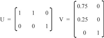
Next the table is extended with an alternative production method for the agriculture, which is presented in the colum τ(g2). Suppose that 9 bales of corn are generated with the technique τ(g1) and 3 bales of corn are generated with the technique τ(g2). Note that here the condition lg = 20 is abandoned. It is again reasonable to combine these two groups of corn producers in an aggregated branch. In that case the weighing factors are respectively wg1 = 0.75 and wg2 = 0.25. The figure 3 shows the form of the transformation matrices U and V.
Note that the production coefficients in the table 1 form a 2×3 matrix. Apparently the transformation U is already accomplished here. Incidentally, this is also clear from the data, because these show that both production techniques generate the same type of corn. Apparently merely the transformation V of the formula 7 must be performed. The table 2 shows the production coefficients after the aggregation, where the aggregated technique is indicated simply by τ(g). The metal branch remains unaffected.
| agriculture | industry | |
|---|---|---|
| τ(g) | τ(m1) | |
| graan | agg=0.3807 | agm=1.290 |
| metaal | amg=0.03523 | amm=0.6452 |
Now, at the end of this column, a related theme is addressed, namely the foreign trade11. In a previous column a method is sketched to model the foreign trade in an intertwined balance, assuming a single homogeneous foreign country. It concerns a balance in kind. However, it can be useful to separate the foreign trade in all K states, which are involved in trade. For instance, some products i do not have a uniform price on the world market, so that they are imported with a differentiated price pik, depending on the supplying state k (with k = 1, ..., K). The price pik expresses the terms of trade with the state k. The addition of the foreign trade changes the formula 1 for the balance in kind:
(9) x = A · x + η + Σk=1K bk
In the formula 9, bk represents the trade balance with the state k, so the difference of the export ek and the import ik. Note that the trade balance with the state k is a vector, because all common products i can be traded. Thus the mathematical form of the trade balance is bik = eik − iik. When the trade balance for the product i is positive, then a part of the nett product is sacrificed to the export. Therefore less of the product i remains for the interior consumption, namely a quantity ηi = yi − Σk=1K bik. When the trade balance for the product i is negative, then more of it can be consumed than the nett product.
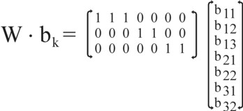
The expression in the formula 9 is actually too ample, because the product i is commonly traded with merely a limited number of states, certainly less than K. A more succinct formula is obtained, when use is made of a matrix of the same kind as U. For, this allows to aggregate all foreign trade with the product i in a simple manner. In order to avoid confusion, this "trade" matrix is called W. The matrix W is filled with vertical (N×1) unit vectors n(i), with nj(i) = 1 for j=i, and nj(i) = 0 for all other j. W has as many colums n(i) as there are states, which are engaged in the trade of the product i. It is naturally convenient and transparent to place these colums n(i) together as a block in W.
In this approach the vector bik takes on the following form: from the top to the bottom, it contains first all components b1k, where the index k counts all states, that are engaged in the trade of the product 1. Next it contains the components b2k, where the index k counts all states, that are engaged in the trade of the product 2. That number probably differs from the number for the product 1. In the same manner the vector bik is filled further, up to and including bNk. Therefore the number of components of the vector bk equals S = (number of states, that trade in product 1) + (number of states, that trade in product 2) + ... + (number of states, that trade in product N) 12. The figure 4 illustrates the matrix W and the vector bk. Thus the formula 9 changes into
(10) x = A · x + η + W · bk
For the foreign trade, the transformation of the balance in kind is fairly straightforward. Suppose for the sake of convenience that the industry and the consumers of ηi pay the price pi for the product i. Furthermore, assume that the product i in the foreign trade with the state k has a price pik. Combine these foreign product prices into a diagonal matrix Π, so that the elements pik have the same order as the components bik. Finally, let ρi be the average price of the sales xi, and insert these N average prices into the diagonal matrix R. Then the value balance is given by13
(11) R · x = AM · P · x + P · η + W · Π · bk
Finally, note that the total trade balance should not be negative for a long time. The global equilibrium requires, that the total trade balance of each state is zero, on average. In other words, one must have Σi=1N Σk=1S Wik × pik × bik = 0.