A dynamic model of growth and conjuncture

First insertion on Heterodox Gazette Sam de Wolff: 7 august 2013

In previous columns attention has been paid to dynamical phenomena such as the economic growth and the conjuncture. The present column describes a multiplier-accelerator model, which is able to describe both phenomena at once. The model has been invented and published by the famous economist Luigi L. Pasinetti. It turns out that some simple mathematical formulas for the national income and for the investments with time lags are sufficient for the generation of a dynamic behaviour, which closely resembles the real economy. At the same time it becomes clear, that a successful model simulation does not imply, that the reality is actually explained and understood.

The now following text has been published before in the provisional reader Vooruitgang der economische wetenschap. This paragraph is based on the book Growth and income distribution by L.L. Pasinetti¹. In a previous column about conjuncture cycles several schemes have been discussed with regard to the available theories and models. The findings of Pasinetti belong to the category of the multiplier-accelerator models. Besides, it is a one-sector model, because merely the aggregate quantities at the national level are computed.

The accelerator formula describes how the economic growth becomes an incentive for the entrepreneurs to invest. It suggests a macro-economic relation. Its mathematical form is

(1)     ΔK(t) = κ × ΔY(t)

In the formula 1 ΔY(t) is the growth of the national income Y during the time interval between t-Δt and t. The capital accumulation ΔK(t) is the investment I(t), which is chosen by the entrepreneurs at the time t. Apparently the assumption is, that this investment will be proportional to the absolute growth of the incomes. The proportionality constant κ is called the capital coefficient. Loyal readers will recognize this coefficient from the column about the model of Harrod-Domar, which describes the economic growth. The difference is, that the formula 1 is expressed in differences and not in differentials.

Usually ΔY(t) is not yet known at the time t. Therefore the entrepreneurs must base their investments on the expected growth. Suppose, that they do know the growth from the previous period, at the time t-Δt, Than it is obvious that they will calculate their estimate by means of the formula

(2)     ΔY_V(t) = ΔY(t − Δt) = Y(t − Δt) − Y(t − 2×Δt)

The formulas 1 and 2 show, that the behaviour of the entrepreneurs (the acceleration) can be approximated by the formula

(3)     I(t) = κ × (Y(t − Δt) − Y(t − 2×Δt))

It is worth while to compare the formula 3 with the investment theory of Kalecki, which has been discussed in a previous column. In the investment function I(t) of Kalecki the entrepreneurs act on the changes in the rate of profit r = ΔP/ΔK, where ΔP is the change of the profit. The formula 3 is a bit sloppier, because merely ΔY is considered, which contains both a profit and a wage component. In other words, the entrepreneurs would also invest, when the wages W rise but not the profit P. Furthermore, the investment function of Kalecki contains an autonomous term, which models the replacement of the scrapped equipment. Apparently the formula 3 represents merely the nett investments, and the investments for replacements have been discarded.

The multiplier part of the theory is caused by the consumption. The consumption is represented by the consumption function

(4)     C(t) = C_A + c × Y(t − Δt)

In the formula 4 c is the marginal consumption quote, and C_A is the autonomous consumption, which is present, irrespective of Y. In the case Y≤0 the consumers break into their savings, or they take a credit. Note, that the consumers adapt their behaviour to the national income with a lag Δt. The consumption function is also known from the theory of Kalecki, where she represents the behaviour of the capital owners. In the present model of Pasinetti the consumption of the capital owners and the workers is aggregated.

The national income is generated in the form of added value during the production of the consumer and capital goods. In formula this is

(5)     Y(t) = C(t) + I(t)

Since it is always supposed that the markets clear, all consumer goods are consumed. Therefore the term I(t) must equal the savings S(t). The national income always changes in such a manner, that I(t)=S(t) is satisfied. But these "ex post" savings are not equal to the amount, that was planned "ex ante" by the households, namely Y(t-Δt) − C(t)!²

It may be useful to sketch briefly in a paragraph why the multiplication occurs here. Assume for convenience, that the investments are constant (I(t) = I_A). Then, according to the formulas 4 and 5 the economic growth equals Y = (C_A + I_A) / (1 − c). It is obvious that the factor 1-c in the denominator is less than 1. Its inverse is called the multiplier, because the investment I_A (and incidentally also C_A) has a manifold reappearance in the national income³.

For the general case combining the formulas 4 and 5 yields the formula

(6)     Y(t) = C_A + (c + κ) × Y(t − Δt) − κ × Y(t − 2×Δt)

The formula 6 shows that, dependent on the situation in the past and the c- and κ-values, the national income Y(t) will develop in very different ways. The model of Pasinetti generates the dynamical behaviour in an endogenous manner, without the need for external shocks. The dynamics originates purely from the fact, that both the consumers and the producers react with a lag on the economic developments. Pasinetti has shown by means of mathematics, that four types of fluctuations can be distinguished. He derives four mathematical formulas, which each represent one of these types. However, for this column it suffices to consider four examples, where each example is characteristic for one of the types.

In all examples the autonomous consumption C_A is equated to 10, and the marginal consumption quote c equals 0.9. The multiplier 1/(1 – c) = 10 has the effect, that the autonomous consumption in the national income is enlarged to 10×C_A = 100. The fluctuations develop around this value of Y. Therefore it seems reasonable to perform all computations with the initial conditions Y(0) = 99 and Y(Δt) = 101.

The damped oscillation

In the first example the capital coefficient κ equals 0.8. The difference equation becomes

(7)     Y(t) = 10 + 1.7 × Y(t − Δt) − 0.8 × Y(t − 2×Δt)

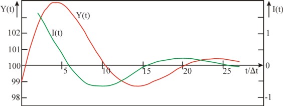
Next the development of the national income and the investment can be computed by means of the formula 7. The result is shown in the table 1 and in the figure 1.

Figure 1: National income Y and investment I as a function of time t

In this example the national income behaves like a sinoid, which oscillates around the value 100. The first crisis occurs at t = 4×Δt, and the second one at t = 24×Δt. Apparently the period of the cycle equals 20×Δt. It is clear that many derived variables can be computed from the table 1. The investment I(t), which is also included in the table 1 and is computed by means of the formula 3, has the same period as Y(t). It already starts to fall at a time 5×Δt before the crisis, it crosses zero shortly after the crisis as well as shortly after passing the bottom of the recession. The consumption C(t) equals Y(t) − I(t), and can be computed from the table 1, if desired. It is striking, that the national income during the first boom reaches a value of 103.87, and in the second one 100.42. This decrease shows, that the oscillation is damped and will extinguish gradually.

Pasinetti has derived a functional relation for the simulated type of fluctuations:

(8)     Y(n×Δt) = C_A + A × κ^n/2 × cos(n×θ + φ)

The quantities A and φ are constants, which are fixed by the choice of the initial conditions (namely Y(0) and Y(Δt)). The damping is caused by the term κ^t/2, of course provided that κ<1. In the formula 8 the angle θ must satisfy

(9)     cos(θ) = (c + κ) / (2×√κ)

This relation leads to the requirement, that κ and c satisfy (κ+c) / (2×√κ) ≤ 1, and indeed κ=0.8 and c=0.9 fulfil this condition. According to the formula 9 θ in the example equals 18.13^o, so that during the period of 20×Δt indeed a total angle of 360^o is completed.

The exploding oscillation

In the second example the capital coefficient κ equals 1.2. The difference equation becomes

(10)     Y(t) = 10 + 2.1 × Y(t − Δt) − 1.2 × Y(t − 2×Δt)

The development of the national income can be computed by means of the formula 10. The result is presented in the table 2 and in the figure 2.

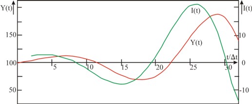
Figure 2: National income Y and investment I as a function of time t

The national income is also in this example a sinusoid, which displays a time dependency with similar oscillations as the first example. However, the amplitude of the sinus curve behaves completely different. The national income reaches a value of 112.00 in the first boom (at t=7×Δt), en an impressive 186.83 in the second one (at t=29×Δt). The oscillation explodes for this type, and in the ensuing recession she will even fall to Y=0. It is obvious, that no society can endure such extreme changes without damage. The state will be forced to intervene already during the first cycle with regulations⁵.

According to Pasinetti also the exploding oscillation is described by the formulas 8 and 9. Since now one has κ>1, the term κ^n/2 causes indeed an explosive rise of the amplitude. According to the formula 9 θ in this example equals 16.56^o, so that now almost a time 22×Δt is needed to complete the total angle of 360^o.

The converging decay

In the third example the capital coefficient κ equals 0.4. The difference equation becomes

(11)     Y(t) = 10 + 1.3 × Y(t − Δt) − 0.4 × Y(t − 2×Δt)

The development of the national income can be computed by means of the formula 11. The result is presented in the table 3 and in the figure 3.

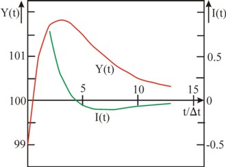
Figure 3: Y and I as a function of time t

The national income exhibits in this example a decay, which converges to the value of 100. Apparently here the difference equation does not generate a conjuncture, but a long-term change. However, the numbers in the table 3 do show, that the decay does not proceed in a balanced manner⁶.

Pasinetti has derived a functional relation for this simulated type of change:

(12)     Y(n×Δt) = C_A + A₁ × x₁ⁿ + A₂ × x₂ⁿ

The quantities A₁ and A₂ are constants, which are fixed by the choice of the initial conditions(namely Y(0) and Y(Δt)). The x-terms are determined by κ and c:

(13a)     x₁ = (κ + c)/2 + √((κ+c)²/4 – κ)
(13b)     x₂ = (κ + c)/2 − √((κ+c)²/4 – κ)

Here x₁ and x₂ are real numbers, so that the expression below the square-root can not be negative. Therefore κ and c must satisfy the requirement κ+c ≥ 2×√κ. Moreover the formula 12 represents only a converging decay, as long as x₁ and x₂ are both less than 1. Here x₁ is the crucial term, because x₁>x₂. In other words, it is required that (κ + c)/2 + √((κ+c)²/4 – κ) < 1. The square-root is non-negative, so that one has κ+c < 2. Indeed κ=0.4 and c=0.9 satisfy both requirements. The insertion of this κ and c in the formulas 13a-b yields for x₁ and x₂ respectively the values 0.8 and 0.5. When some time has passed, Y–C_A is dominated by A₁ × x₁ⁿ, and therefore it decreases by a factor x₁=0.8 during each following step Δt. Then x₁ has become the rate of decay.

The exponential growth

In the fourth and last example the capital coefficient κ equals 1.8. The difference equation becomes

(14)     Y(t) = 10 + 2.7 × Y(t − Δt) − 1.8 × Y(t − 2×Δt)

The development of the national income can be computed by means of the formula 14, The result is presented in the table 4 and in the figure 4.

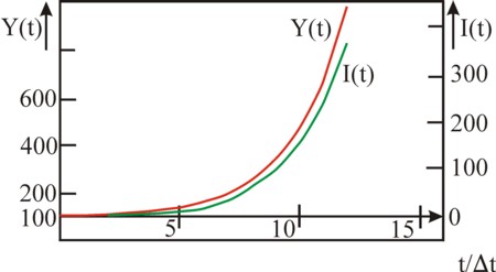
Figure 4: Y and I as a function of time t

The national income exhibits in this example an exponential growth. The difference equation does not generate a conjuncture for this type either, but a long-term growth. Due to the arbitrary initial conditions Y(0) and Y(Δt) this growth will not be stable either, just like the decay in the preceding paragraph⁷.

According to Pasinetti also the exponential growth is described by the formulas 12 and 13a-b. Since for this type at least the largest square-root must satisfy the demand x₁>1, the term x₁ⁿ causes indeed an explosive rise of the amplitude. The requirement implies that (κ + c)/2 + √((κ+c)²/4 − κ) > 1. In other words, √((κ + c)² − 4×κ) > 2 − (κ+c). It turns out, that this is only possible when 2 − (κ + c) is not positive. So the requirement κ+c≥2 must be satsified. Indeed κ=1.8 and c=0.9 satisfy this demand, and κ+c ≥ 2×√κ as well.

Insertion of this κ and c in the formulas 13a-b yields for x₁ and x₂ respectively the values 1.5 and 1.2. After some time Y–C_A is dominated by A₁ × x₁ⁿ, and therefore it increases by a factor x₁=1.5 for each following step Δt. Then x₁ has become the rate of growth. The rate of growth depends on the savings quote s=1–c and on the capital coefficient κ. That reminds of the formula for the growth rate in the Harrod-Domar model (see the pertinent column). However, the functional dependency x₁(c, κ) is more complex than the Harrod-Domar growth rate g_w.

Evaluation of the dynamical model of Pasinetti

In the four preceding paragraphs it turned out that the interaction between the accelerator principle and the multiplier can lead to completely different processes of change. The series of examples shows how the growth can be stimulated more, according as the capital coefficient κ is raised further. A larger κ implies, that the producers must make considerable investments, when the demand for their products increases. This is expressed in the formula 3, which for the chosen initial conditions reduces to I(2×Δt) = 2×κ. All those investments together will push the consumptive demand further upwards, due to the amplifying effect of the multiplier (which depends on the consumper quote c).

The quantitative effect of the multiplier determines, whether the demand increases sufficiently in order to seduce the producers to again make extra investments. This shows how for a damped oscillation the first wave of investments is so small, that it is unstable and withering. The exploding oscillation shows a first wave of investments, which durably improves also the later consumptive demand. Yet here sometimes periods of a feeble trust return, which cause temporary economic slumps. This gives an unstable character to this type of economy. Only the exponential growth displays a durable improvement.

At first sight it is impressive, that both the conjuncture and the long-term growth can be reproduced with one difference equation. However, Pasinetti is correct in pointing out a contradiction, which emerges here. The equation of the conjuncture requires κ+c ≤ 2×√κ, whereas the equation for the continuous growth requires exactly the opposite, so κ+c ≥ 2×√κ. The two types of change seem to exclude each other. Pasinetti solves this problem by supposing, thath social processes lead to perpetual changes in the values of the quantities κ and c.

Suppose for instance, that the economy exhibits the conjunctural behaviour of the damped oscillation. A technical invention could lead to a sudden rise of κ to 1.8, so that the economy switches to an exponential growth. After some time another change could occur, for instance a fall of the consumer quote due to the rising national income. Etcetera. The disadvantage of the solution of Pasinetti is, that then the multiplier-accelerator approach must be combined with knowledge about the changes in κ and c.

An alternative explanation is given by H.J. Sherman⁸. He notes, that not only do the recent events affect the human behaviour, but also the distant past. Therefore the consumption- and investment-functions in the formulas 4 and 3 must in fact also contain terms for the times t − 2×Δt, t − 3×Δt etcetera. The adapted equations occasion business cycles with a behaviour, which is a mixture of the time dependency in the four examples.

A striking hallmark of the multiplier-accelerator model is, that the dynamics is endogenous, that is to say, inherent for the economic system. In the previous column about the conjuncture it has been explained, that many other categories of theories are available. Some of those theories state, that the conjuncture is caused by the technological progress⁹. Also the model of Sam de Wolff belongs to this category. The rising productivity would occur in shocks, which cause waves. Since such a change of technique will lead to a changing capital coefficient (generally a rise), the multiplier-accelerator model can not describe it.

This statement deserves some reflection. Indeed the changes of the technique can lead to economic oscillations. Now in this column a model has been introduced, which can mimic the oscillations, but couples this to a completely different interpretation. Apparently the optical similarity between a model and the reality is not a guarantee, that the assumptions in the model are true. In such a case the model does not give an insight into reality, and it is just an empirical parametrization. The extraordinary mathematical beauty of the multiplier-accelerator model must not be a reason to adhere to economic chimeras!

Furthermore it is striking, that the multiplier-accelerator model does not pay attention to the development of the prices. And the wages and prices have merely an indirect effect, through the national income. Therefore the model is not able to explain oscillations due to wage pressure, or in general due to the squeezing of the profit (the so-called profit-squeeze). The model can merely account for the wage pressure or the profit squeeze in an indirect manner, namely when a relation could be found between on the one hand the national income and the investments, and on the other hand the wages and the profits.

In general the conjuncture and the growth will naturally be the result of a variety of factors. Even when the poly-causal theory is used, it will still not be possible to calculate all those effects in a factual way. Therefore the explanation of the economic dynamics remains a task for experts. Each case requires its own study in order to clarify the dominant and deciding mechanisms in the concerned situation.

1. See the paragraphs 11.5 and 11.6 in the provisional reader Vooruitgang der economische wetenschap (2011, uitgeverij E. de Bibelude) by E.A. Bakkum and chapter III in Growth and income distribution - Essays in economic theory (1974, Cambridge University Press) by L.L. Pasinetti. The contents of the reader is now almost completely copied to this portal, sometimes in an improved version. (back)
2. See p.53 of Growth and income distribution. (back)
3. For after a repeated application of the formula 4 one finds the formula Y(t) = c^N × Y(t − N×Δt) + (C_A + I_A) Σ_n=0^N-1 cⁿ. For a sufficiently large N c^N is approximately zero, and the summation is approximately equal to (1-c)^-1. (back)
4. See her and for the following the chapter III of Growth and income distribution. (back)
5. This was already clear a century ago, although the economists were reluctant to admit it. Thus Herman Heijermans writes in his novel Diamantstad (p.165): Why would we be despondent, as long as we have power. We have the power, here, everywhere, we the workers, we only! We have the power, when we stand shoulder to shoulder, head to head, heart to heart! We, we only, when we are united, united till the death, preach the struggle without mercy, an eye for an eye, a tooth for a tooth, because we are never pardonned - no pardon, no justice! For centuries we were a flock, a kicked, maltreated, defenceless flock. (back)
6. The warranted decay would require, that the capital and the national income have the same rate of decay. In formula this is ΔK/K = ΔY/Y. The relation ΔK/ΔY = K/Y should be satisfied, that is to say, the marginal capital coefficient κ would equal the average capital coefficient. Of course the producers can adopt this as a desirability. However, the economic development can not be forced to obey this rule, because it can not be reconciled with the inintial conditions Y(0)=99 and Y(Δt)=101. One sees for instance in the table 3, that ΔY becomes already negative between the times 3 and 4, whereas ΔK becomes negative only at the time 5. (back)
7. The loyal reader will notice, that this variety of the model of Pasinetti is similar to the national income growthmodel, which has been discussed in the column about dynamical one-sector models. (back)
8. See p.155 of The business cycle (1991, Princeton University Press) by H.J. Sherman. (back)
9. Therefore Louis Paul Boon writes in his novel De kapellekensbaan with a fine sense of irony (p.236): in science and reason, in the understanding of all what still has been obscure to the people, there laid thestarting point towards a happier humanity. And he, with his discovery, would bring more happiness and welfare than all unions together: the others quarreled today and rebelled tomorrow and revolted the next day ... but no matter how one tossed and turned, the lower classes would pay the broken pots ... the lower classes are the milkcow, for instance now I must pay the wood ... And terrified he continued to stammer, because now still he had, unwittingly, addressed money: presently the people might think that he had come for that. (back)