Alternative scales of the utility for monetary incomes
First insertion on Heterodox Gazette Sam de Wolff: 21 october 2013
E.A. Bakkum is a blogger for the Sociaal Consultatiekantoor. He loves to reflect on the labour movement.
In a preceding column it has been explained how according to Van Praag and Ferrer-i-Carbonell the income satisfaction question yields an indicator for the utility of the personal income. The indicator can be measured on an ordinal scale by means of the ordered probit method. The present column describes how the cardinal probit yields an alternative scale. Besides, the income evaluation question is discussed, which measures the utility for an arbitrary income. This indicator can also be scaled, at choice, in an ordinal or cardinal manner, by means of the least squares method. The scales are applied to the GSOEP collection of empirical data. The results show, that the satisfaction of a person may drift.
The cardinal probit method of scaling
The column, which has just been mentioned, introduces a frame for the scaling in studies of the preferences of households1. The present column elaborates on this, so that they are affiliated, and form a single unit and a mutual supplement. The contents is again copied from the book Happiness quantified by Bernard van Praag and Ada Ferrer-i-Carbonell2. First the cardinal scale of the income satisfaction question (in short ISQ) will be discussed here. It is somewhat confusing, that she is also called the financial satisfaction question (in short FSQ). The question yields an indicator of the satisfaction and the personal utility, which is derived from the personal income. The reader may remember how in the affiliated column the indicator was used with an ordinal scale, although it was validated with a cardinal latent dimension.
For the sake of convenience the same income satisfaction question is used as in the affiliate column: "How satisfied are you today with your household income?". The individual can choose between five answers: "not at all", "moderate", "sufficient", "good" and "very good". It is convenient to transform these measured values of the indicator U into numbers, respectively 1, 2, 3, 4 and 5. Now contrary to the ordered probit method it is assumed, that the length of the intervals between the measured values are identical. In other words, the answers are interpreted in a quantitative way. Van Praag and his collaborators have shown in various publications, that the individuals indeed implicitely apply a quantitative scale3.
The assumption implies, that for instance individuals with the answer 3 mean in fact a value somewhere between 2.5 and 3.5. They round off their preference to the nearest answer. In the affiliate column it is stated, that such a scale contains more information, and thus performs at a higher level than the ordinal one. For purely mathematical reasons it is convenient to transform the scale again, now into 0, 0.25, 0.5, 0.75 and 1. That is to say, the range of values of the indicator U is restricted to the interval [0, 1]. Again a couple function is wanted, which connects U to the income Y. Due to the cardinality it is no longer necessary to employ a latent model equation.
The equation U = α × ln(Y) is an obvious choice, where ln(.) is the function of the natural logarithm. On reflection she is not really suited, because in this formula the range of values of U is unbounded. The couple function must yield values in [0, 1]. Already in 1968 Van Praag proposed the following couple function4
(1) U = Ψ(ln(Y)) = ∫-ωln(Y) ψ(x) dx
In the formula 1 -∞ is the symbol for negative infinity. The function ψ(x) is positive and normalized to 1. So she is a probability density function. Therefore Ψ(ln(Y)) is the cumulative distribution function.
This approach lends itself well to the present problem. Van Praag and Ferrer-i-Carbonell prefer the Gaussian or normal distribution, with E(ln(Y)) = μ as its expectation value and E((ln(Y) − μ)²) = σ² as its variance. For this case the cumulative distribution function has the symbol Φμσ. A linear transformation can bring the function Φμσ(ln(Y)) in its definite form5
(2) U = Φ01(α × ln(Y) + β)
It is important to realize, that here the probability function Φ01 does not play a stochastic role. She is merely used because of her convenient form, which agrees well with the empirical data. Your columnist hopes, that with this warning the reader will not be confused during the remainder of the present argument. Namely, the normal distribution will appear a second time in the model, now with a stochastic meaning. This happens, because the answers U are discrete (namely, the five alternatives of choice). Therefore the probit method must be applied also in the cardinal approach.
In the affiliate column it turned out, that the individuals do not behave according to a functional relation, such as in the formula 2. They have their own preferences, depending on their attitude in life, obtained by their formation and experiences. That personal preference is modelled by means of the stochastic variable ε, which has a normal distribution (the reader remembers, that this idea was proposed by Quetelet). Thus the model equation gets her final form
(3) U = Φ01(α × ln(Y) + β + ε)
It is assumed, that the variable ε is distributed over the individuals in a purely arbitrary manner. That is to say, its expectation value E(ε) equals zero. In the affiliate column the variance σε² of ε (the spread in its values) could be equated to 1. Unfortunately this assumption can not be made in the cardinal probit method. For such a scaling of ε would influence also the constants α and β, and thus undermine the validity of the formula 3 (μ=0, σ=1). Therefore σε remains present as an extra model parameter, besides α and β. No rose without a thorn.
It is fortunate that the boundaries νj of the intervals of U are not model parameters, such as in the ordinal method. Now one simply has νj = j − 1/8 for j = 0.25, 0.5, 0.75 en 1, and ν0 = 0 and ν1 = 1. The interval length of the choice alternatives is fixed at 0.25. The boundaries express, that the individuals round off their answer to the nearest alternative. The model parameters α, β and σε can be determined by means of the maximum likelihood method, which has been introduced in the previous column. The estimate maximizes the probability, that the measured values of the indicator do indeed occur.
It is straightforward to show, that the probability to measure U = j (j=0, 0.25, 0.5, 0.75, 1) equals6
(4) Pr(νj < U ≤ νj+1) = Φ0σ(Φ01-1(νj+1) − α × ln(Y) − β) − Φ0σ(Φ01-1(νj) − α × ln(Y) − β)
In the formula 4 Φ01-1 represents the inverse function of the cumulative normal distribution. She is called the probit link function. The values of the probit link can be read from a table7.
The empirical data are a set of data with regard to the complete sample of individuals, say numbered k = 1, ..., K. The probability to obtain this set of data is the product of the K probabilities Pr(νj < Uk ≤ νj+1) for the answers of the separate individuals. The maximum likelihood method aims to find the α, β and σε, which maximize the product of probililities. Thus after the ordered probit method now also the cardinal probit method has been explained.
An illustration of the cardinal probit method
It is clarifying to illustrate the cardinal probit method by means of empirical data. First, the figure 1 shows how the same collection of measured points as in the affiliate column is modelled in the cardinal probit approach. See also the figures in that column. The black dots represent the measured values. The red curve is the link function of the model, which describes the satisfaction. In the figure 1a the satisfaction follows the cumulative normal function. The blue horizontal lines are the boundaries of the satisfaction answers. The figure 1b shows the same objects, but after the transformation with the probit link. Now the vertical range [0;1] is stretched to <-∞;∞>.
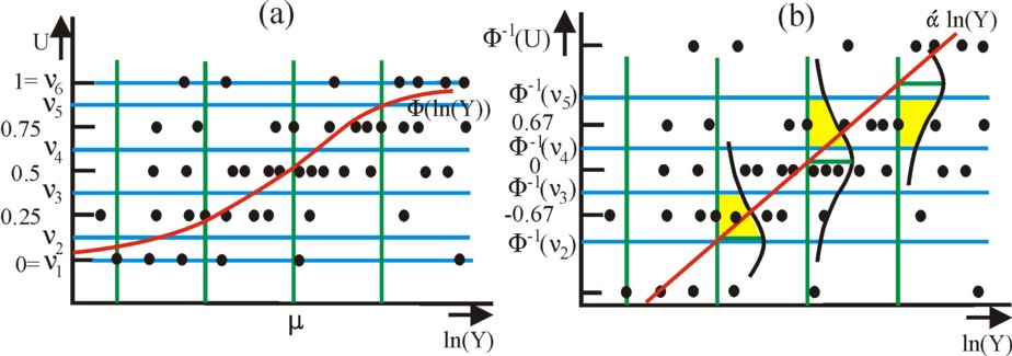
Figure 1: measured points andlink function
Figure (1a): cumulative normal function; figure (1b): idem after transformation with the probit link.
The blue horizontal lines are the boundaries of the satisfaction.
The yellow surfaces represent the probabilities that the point on the green lined is measured.
Even more interesting is the analysis, which Van Praag and Ferrer-i-Carbonell have made of the German socio-economic panel survey (in short GSOEP) for the year 1997. In this collection of data the indicator of the ISQ has a scale with 11 values (instead of 5, such as in the preceding paragraph). Moreover, more independent variables are available, so that the formula 3 changes into
(5) U = Φ01(α × ln(Y) + β × ln(G) + γ + ε)
In the formula 5 G represents the number of members in the household. The estimation with the maximum likelihood method yields α = 0.342, β = -0.102, γ = -2.524 and σε = 0.466. The reader may want to perform his own computations with this result. For instance, suppose that a person behaves precisely according to the general trend. Then one has ε=0. Furthermore, suppose that the person is "sufficiently" satisfied with his own income. Then one has U=0.5, and the formula 5 has the form Y = 1600 × G0.3. This suggests, that in GSOEP the income is stored as the monthly income in German Marks8.
Or consider the following computation: suppose again that the individual is "sufficiently" satisfied. This means that the satisfaction lies between the boundaries 0.45 and 0.55. This corresponds to a probability Pr(0.45 < U ≤ 0.55), which can be translated with the help of the probit link in Pr(-0.13 < 0.342 × ln(Y) − 0.102 × ln(G) − 2.524 + ε ≤ 0.13). Suppose that the individual is single (G=1) with a wage Y=1600. Now the probability is Pr(-0.13 < ε ≤ 0.13) = 0.22 9. In other words, there is a probability of 78%, that according to the general trend (namely 0.342 × ln(Y) − 0.102 × ln(G) − 2.524) the individual ought to be "sufficiently" satisfied, but actually classifies himself in another U category. This computations shows the extent of the spread in personal preferences. The trend gives an indication, but not real life.
The income evaluation question as an indicator
Ordinal approach
The income evaluation question (in short IEQ) is an alternative indicator instead of the ISQ indicator. The IEQ indicator consists actually of six questions. Six values of statisfaction are offered to the individual: "very low", "low", "insufficient", "sufficient", "good", and "very good". The individual must for each value indicate, what in his perception is the height of the corresponding income. This questionnaire yields six values for the IEQ indicator, say ηj for respectively j = 1, 2, 3, 4, 5, and 6. It is clear, that the IEQ indicator yields more information than the ISQ indicator. Since there are six measured values (items), there must also be six scales.
The IEQ indicator can by scaled in both an ordinal and cardinal way. The present column wil explain both scalings, starting with the ordinal one. First note, that in this case the answers have a continuous scale. The individual does not need to restrict his choice to a handful of alternatives, but may fill in any conceivable monetary sum ηj (a positive real number). In this situation the probit method is not needed. And the maximum likelihood method can be replaced by the simple least-squares method.
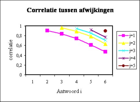
Figure 2: correlations between deviations (i,j = 1-6)
It is obvious that in the IEQ the differences between the monetary sums ηj are known. The ordinal character stems from the fact, that no quantitative assumptions are made with regard to the distances between the six satisfaction values "very low", ..., "very good". In the ordinal approach the model equation is
(6) ln(ηj) = αj × ln(Y) + βj × ln(G) + γj + εj
The reader sees, that in this model each quantity ηj has her own model parameters. The quantity εj is naturally again the deviation of the measured value with respect to the general trend. She expresses the personal attitude of the individual.
In a model equation such as the formula 6 the parameters are estimated by means of the well-known least-squares method10. That method yields estimations for the parameters αj, βj and γj. It turns out, that they are all positive, which stimulates some reflection. Apparently for an arbitrary income the judgement of the corresponding satisfaction depends on the individual situation (income and size of the family). Furthermore note, that now β is positive, because the individual has included the effect of the family size in his answer ηj. An individual with a large family will prefer a higher income than a single man, in order to give the answer "sufficient".
The dependency of the judgement on the situation is called the preference drift. When someone enters a new situation, then he will adapt the judgements ηj in a corresponding manner. Individuals can probably make a reasonable estimation of the satisfaction with an income, which deviates little from their own income. According as the situation becomes more extreme, for instance "very low" or "very high", then the answer will probably be less reliable. It is necessary to speculate. Indeed it turns out, that in the GSOEP data the correlation between εi and εj diminishes, according as i and j are farther apart. This phenomenon is shown in the figure 2, which presents the correlation coefficients of the two deviations11.
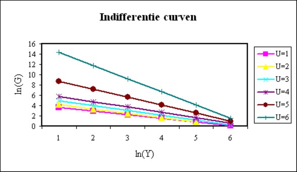
Figure 3: Personal indifference curves
For the sake of completeness the figure 3 shows the formula 6 for all j = 1, ..., 6, based on the estimations with the GSOEP data. Here, for the sake of convenience it is assumed, that the individual behaves according to the trend, and thus has an εj equal to zero. The individual earns Y=1600 (say, DM per month), and is single (G=1). The lines in the figure 3 correspond to answers ηj = 1000, 1200, 1500, 1900, 2600, and 3600 for respectively j = 1, 2, 3, 4, 5 and 6, which have been selected at random by your columnist. The lines can be interpreted as the indifference curves of the individual. Note that the situation of the individual implies ln(G)=0, which is completely to the right in the figure 3.
The figure 3 is intriguing. For, suppose that the individual experiences a fall of the income Y. The indifference curves show, that then for the same satisfaction value j the individual will accept a larger family. It is obvious, that in this way the income per person in his household will fall. For instance the answer η1 = 1000 at G=2 implies a monetary sum of merely 500 per person. Therefore the individual apparently reduces his demands in the situation of a lower income, and is sooner satisfied with his income. In this case the indifference curves take into account the changing perception of the individual. In a sense they are dynamic here.
The reduction of the needs due to a falling income is most striking in the situation with the highest satisfaction values. The reader sees how for the case with the answer η6 = 3600 a falling income will induce the individual to expand his family and household appreciably, which will cause an equally large fall of the income per person. Due to the falling income of the individual η6 = 3600 suddenly seems to promise a relatively larger financial richness. That allows for a larger family or household.
The income evaluation question as an indicator
Cardinal approach
In the cardinal approach it is assumed, that the intervals between the satisfaction values "very low", "low", "insufficient", "sufficient", "good", and "very good" are equal. This assumption has already been made plausible in the preceding text. Moreover, the range of satisfaction- or utility-values is restricted to the interval [0, 1]. Both demands are satisfied by transforming the six satisfaction values into 1/12, 1/4, 5/12, 7/12, 3/4 en 11/12 (or into (2×j − 1) / 12 with j = 1, ..., 6).
The cardinal method requires, that the degree of satisfaction is also known in the intervals between these six values. Almost the same link function is used as in the formula 5, namely
(7) U(k) = Φμ(k)σ(k)(ln(η)) = Φ01((ln(η) − μ(k)) / σ(k))
Here Φμ(k)σ(k) is again the cumulative function of the normal distribution. The symbols U(k), μ(k) and σ(k) indicate, that they characterize the individual k in the data collection. For, each individual gives a special characteristic form to his utility function. The IEQ allows to estimate the parameters of this personal function.
The expectation μ(k) = E(ln(η)) is computed by means of the integration with φμ(k)σ(k)(ln(η)) as the probability density function of the normal distribution. This quantity μ(k) can be estimated with the expression m(k) = Σj=16 (ln(ηj(k)))/6. Here ηj(k) represents the answers of the individual k. The values of ln(ηj) have as their average simply m(k), because the values Uj(k) have just been chosen at equal distances. In the same way the variance σ²(k) can be estimated by s²(k) = Σj=16 (ln(ηj(k)) − m(k))² / 5 12. The reader sees here the wealth of information, that is contained in the IEQ. Elsewhere Van Praag calls μ the natural unit of the variabele, and σ² the welfare sensitivity13.
In the cardinal approach the model equation is a regression formula
(8) m(k) = α × ln(Y(k)) + β × ln(G(k)) + γ
In the formula 8 Y(k) and G(k) are respectively the income and the family size of the individual k. The least-squares method can be applied to the K equations in order to estimate the model parameters α, β and γ. Apparently in this case the cardinal approach needs less model parameters than the ordinal one. It can be estimated from the GSOEP data, that α = 0.527, β = 0.121, and γ = 3.611.
The quantity s² can also be put in the form of the formula 8. Then one finds, that this welfare sensitivity does not exhibit a clear trend. Therefore Van Praag and Ferrer-i-Carbonell put α = β = 0, and then find s² = γ = 0.453. Apparently in the data collection of the GSOEP the welfare sensitivity spreads in an arbitrary way around this average value. This completes the cardinal analysis of the iEQ.
Note that now the formula 7 can be used to calculate the answers according to the trend for an individual in a given situation. Suppose that the situation is Y=1600 and G=1 (similar to the ordinal example). Then one has m=7.50, and thus em = 1810. The six answers ηj are 960, 1330, 1630, 1980, 2430 and 3350 for respectively j = 1, ..., 6. This information is not available in the ordinal approach.
Welfare functions
In fact the formula 7 represents the welfare function of an individual. The function expresses the judgement of the individual k with regard to the utility of various incomes. In the short run the function is fixed, and μ(k) and σ(k) are constants. Van Praag and Ferrer-i-Carbonell call this the short-term or virtual welfare function.
In the long run μ(k) can change, because the individual k may receive a different income Y or the family size G may change. Now μ(k) must again by computed with the formula 8. Insertion of that formula into the formula 7 yields14
(9) U'(k) = Φμ'(k)σ'(k)(ln(η))
In the formula one has 9 μ' = (β × ln(G) + γ) / (1 − α) and σ' = σ / (1 − α). The function U'(k) is called the long-term or real welfare function.
The form of U'(k) is mainly determined by the welfare sensitivity σ', which for the GSOEP data is apparently equal to 2.11 × σ. For this implies, that the long-term function U'(k) increases slower with ln(η) than the short-term function U(k) does. In other words, according to the short-term function a change in the income will have a larger effect on the satisfaction than will really be the case in the long run (in retrospect). In the long run the effects turn out to be moderate. There is a process of habituation in the new situation, and one gets accostumed. The reader may recognize this feeling. A poor man acquiesces in his misery, whereas the rich want more. According to your columnist this is the preference drift in an alternative form (even though this is not stated by Van Praag and Ferrer-i-Carbonell).
Perhaps the reader is somewhat confused by the present column. That would be understandable. It is worth remembering two conclusions. Firstly, the income satisfaction question (ISQ, FSQ) shows, that people have very different needs and expectations with regard to their income. This is relevant for politics, because apparently each group with a given level of (dis-)satisfaction has a large diversity in their personal backgrounds (living conditions). Incidentally, merely the cardinal approach yields this information, not the ordinal one. The cardinal approach is also indispensable for acquiring information about the spread of the preferences for the income evaluation question (IEQ). However, all scaling methods clearly reveal the tendency, that satisfaction increases, according as the income increases.
Secondly, the IEQ shows, that after a change of the income the people get used to the new situation. In the long run the emotions weaken. However, it must not be forgotten, that in all decisions the first emotion is decisive15. And finally it can be concluded, that the scaling of satisfaction provides for a meaningful and fascinating extension of our understanding.
- Michiel Mulder parodies in Het ongrijpbare gelijk van John Winkle the fantasies of the scientist (p.11): When we can tell the world how the morals operate, good heavens, what will we win? We win the same world, Joep, no less than that. Humanity, the conservation of humanity in her present form. Man with his reason ... the start of the individual choice ... the end of the hanger-ons, the presumptuous crowd. (back)
- See chapter 2 in Happiness quantified (2008, Oxford University Press) by B.M.S. van Praag and A. Ferrer-i-Carbonell. (back)
- For instance, this can be observed in the analysis of empirical data by means of the ordered probit method, which is discussed on p.19 of Happiness quantified. There the values of the intervals have been estimated by means of an optimal fit of the model-parameters. The lengths of the intervals between the satisfaction values turn out to be: 0.49, 0.45, 0.56, 0.43, 0.65, 0.84, and 0.65. A more complete confirmation of the assumption can be found in the article The measurement of welfare and well-being - The Leyden approach by B.M.S. van Praag and P. Frijters, in the book Well-being: the foundations of hedonic psychology, scientific perspectives on enjoyment and suffering (1999, Russell Sage). (back)
- See p.16 of Individual welfare functions and consumer behavior (1968, North-Holland Publishing Company) by B.M.S. van Praag. The function has been displayed before in the column about individual preferences. (back)
- A well-known mathematical rule is Φμσ(x) = Φ01((x − μ) / σ). The reader can check this for himself with the definitions of the normal distribution in the affiliate column. The consequence is that Φμσ(ln(Y)) = Φ01(ln(Y) / σ − μ / σ) = Φ01(α × ln(Y) + β), with α=1/σ and β = -μ/σ. (back)
- Namely, due to the formula 3 one has Pr(νj < U ≤ νj+1) = Pr(Φ01-1(νj) < Φ01-1(U) ≤ Φ01-1(νj+1)) = Pr(Φ01-1(νj) < α × ln(Y) + β + ε ≤ Φ01-1(νj+1)) = Pr(Φ01-1(νj) − α × ln(Y) − β < ε ≤ Φ01-1(νj+1) − α × ln(Y) − β). Since ε has a normal distribution, this can be rewritten as Pr(νj < U ≤ νj+1) = Φ0σ(Φ01-1(νj+1) − α × ln(Y) − β) − Φ0σ(Φ01-1(νj) − α × ln(Y) − β). Which had to be proven. (back)
- Your columnist uses the table on p.552 of Introduction to the theory of statistics (1974, McGraw-Hill, Inc.) by A.M. Mood, F.A. Graybill, and D.C. Boes. Any other decent book about statistics will also suffice. For ν = 0, 0.125, 0.375, 0.625, 0.875 and 1 one finds respectively -∞, -1.15, -0.32, 0.32, 1.15, and ∞. The function is mirrored in a symmetrical manner around ν = 0.5. (back)
- It is striking, that Van Praag and Ferrer-i-Carbonell in Happiness quantified do not mention the used unit of the income. (back)
- Namely, Pr(-0.13 < ε ≤ 0.13) = 2 × Φ0,0.466(0.13) − 1 = 2 × Φ01(0.13/0.466) − 1 = 0.22. (back)
- Readers, who are unfamiliar with the least-squares method, can consult any decent introductory textbook about statistics or measurement techniques. For instance an explanation can be found on p.498 of Introduction to the theory of statistics. Incidentally, Van Praag and Ferrer-i-Carbonell state on p.38 of Happiness quantified, that they apply the seemingly unrelated regression (in short SUR). Your columnist is not familiar with this variety of the least-squares method. Perhaps the choice for the SUR is related to the fact, that the six quantities εj are mutually correlated. For these quantities will behave in a similar way for an individual, because they are determined by his or her personal attitude. (back)
- See p.40 in Happiness quantified. (back)
- See for instance p.229 of Introduction to the theory of statistics. The formula on p.40 of Happiness quantified contains a printing error. (back)
- See p.37-38 in Individual welfare functions and consumer behavior. (back)
- For (ln(η) − μ) / σ = (ln(η) − α × ln(η) − β × ln(G) − γ) / σ = (ln(η) − (β × ln(G) + γ) / (1 − α)) / (σ / (1 − α)) = (ln(η) − μ') / σ', with μ' = (β × ln(G) + γ) / (1 − α) and σ' = σ / (1 − α). (back)
- Therefore Willemijn Dicke in Mea can not refrain from a certain self-derision (p.44): The citizens are not interested in the truly important things, certainly not when it concerns affairs in the long run. And when they are interested, they do not really understand it. And such folks are expected to participate in strategic discussions. They merely defend their self-interest, those little people. Merely the elite is enlightened. (back)