Figure 1: LP problem for α
The price of a product can be determined by its scarcity, or by the costs, which must be made for its production. The optimal distribution or allocation of the scarce products is the fundamental concern of the neoclassical paradigm. This question can be solved with the method of linear programming. On the other hand, the relation between the product prices and the production costs is described by the neoricardian model of Sraffa. The construction of input-output tables is a hallmark of this approach. The present column is based on and inspired by the book Vorlesungen zur Theorie der Produktion by the famous economist Luigi L. Pasinetti1.
The neoricardian paradigm derives the prices from the production costs, augmented by a markup for the profit. The Italian economist P. Sraffa has formulated the modern version of this paradigm, by the introduction of a mathematical model for the relation between the prices and the production technique. His model has been explained so often in the Gazet, that here your columnist forgoes this task. If desired the reader can consult the previous column about the choice of the production technique.
In the Gazet most of the columns about the model of Sraffa pertain to the set of production prices. However, the intertwined tables, which are also called input-output tables, are the starting point of the model. In their most simple form the tables represent the quantities of the products, and not their prices. The primary table describes the material distribution of the means of production over the various branches (which is expressed by the word intertwined). Together with the wages and the profit these means of production form the total product Q.
Obviously the society is not very interested in Q, but mainly in the nett product QN, which is available for consumption. That is to say, the size of the nett product must equal the consumptive demand on the market. For a given total product Q the size and the composition of the nett product are determined completely by the applied production technique. The production technique is characterized by two types of coefficients, which together express the demand for production factors.
The production coefficients, indicated by the symbol aij, represent the quantity of the means of production i, which is used during the creation of a unit of end product j. The labour coefficients, indicated by the symbol aj, represent the amount of labour l, which is employed during the creation of a unit of end product j. In matrix notation the production coefficients are simply a matrix A, and the labour coefficients are a vector a. This method of notation is very versatile, when the production is neutral with respect to changes in the scale of production. For then the values of the coefficients are constant.
Now one has for the nett product
(1) QN = (I − A) · Q
In the formula 1 I refers to the unity matrix. When the effective demand on the market equals QN, then its satisfaction requires that the total product has the size:
(2) Q = (I − A)-1 · QN
In the set 2 the upper index -1 refers to the inverse of the matrix within the brackets. Changes in the demand can be satisfied without changes in the technique, but in this case the vector Q must be adapted. This is a striking difference with the neoclassical paradigm, where a change in consumption leads to a shift in the allocation of production factors, and thus to a change of technique.
The amount of the employed labour L in the production is determined by a separate formula, which can be added to the set of equations 1 or 2:
(3) L = a · Q
This is a mathematical inner product, where thus the vector a is horizontal (row vector).
The set 1 shows that the nett product can be enlarged by an increased production. The formula 3 shows that in that case more labour must be expended. The size of L is fairly flexible, thanks to unemployment, and measures such as the adjustment of the labour time and the age for retirement. But finally the size of the population will still impose physical limitations on L, and thus on the increase of Q. The consumptive demand can not be larger than the production capacity. In the long run the rising needs must be satisfied by a transition to another technique with a higer labour productivity.
In the neoclassical paradigm both the consumers and the producers aspire the optimal satisfaction of their needs. The consumers maximize the utility of their income. The producers maximize the profit of their production. In order to relate to the neoclassical paradigm a process of optimization is also introduced in the set 2. The set can be solved with the method of linear programming (LP). Linear programming is an optimization procedure, which for a (historically) available quantity of products searches for their most efficient application. The interested but ignorant reader can find a detailed explanation in the a href="ua120826.html">column about multiperiod optimization.
Succinctly formulated, the present LP problem looks like this:
(4a) maximaliseer Z = p · (I − A) · Q onder de voorwaarden
(4b) (I − A) · Q ≥ QN
(4c) a · Q ≤ L
(4d) Q ≥ 0
In the set 4, Z is the target function of the society. The target function expresses the needs and priorities of the society, and therefore is the core and the reason for existence of the optimization problem. She is the result of the social debate. Even the choice for maximization is questionable. An alternative is the minimization of Z, for instance when Z represents the production costs.
The vector p in Z represents the weighing of the various products. It seems evident to select the product prices as weighing factors. However, on reflection a careful argumentation is needed here. For instance Pasinetti on p.198 of his book prefers to use a target function, which deviates from the formula 4a, namely Z = p·Q. Apparently he wants to maximize the value of the total product, and not (like in the formula 4a) the surplus product (I−A) · Q. Unfortunately, Pasinetti does not explain his choice.
Your columnist does not follow Pasinetti, because the surplus product appears to be more relevant than the total quantity of available utility goods. For the surplus product is the essential factor for the standard of living. In the mathematical sense the formula 4a chooses different weighing factors than Pasinetti, namely p · (I−A) instead of p 2.
In the planned economies of the former Leninist states the application of the LP at the macro level has attracted considerable attention. This approach has been described in the column, just mentioned, about the multiperiod optimization. The East-German economist Eva Müller points out, in her book Volkswirtschaftlicher Reproduktionsprozeß und dynamische Modelle, that the weighing factors in Z are actually time-dependent3. In a realistic LP problem that dependency must be included, which obviously complicates its solution.
This complication is characteristic for the application of the LP problem at the macro level. The consumers determine their effective demand by weighing the market prices of the products against their marginal utility. When now the supply Qi of a utility good i grows with time, for instance in an attempt to realize the optimal situation, then this act will also change the marginal utility. Afterwards, the clearing of the market will only be possible by means of a reduction of the price. Pasinetti, and in his footsteps this column, ignores the change of the marginal utility and of the demand on the market. Perhaps this theme, and the vision of the experts on planning, will be discussed further in a future column. For instance, Eva Müller states in her book, that the optimization is not very sensitive to the form of the target function4.
The inequality 4b implies that the surplus product must be at least as large as the desired nett product. Here the nett product is the consumptive demand, which must definitely be satisfied. This part of the consumptive expenditure is not influenced by the optimization procedure5. The surplus product is limited by the stock of labour L (inequality 4c). But within this natural limitation the means of production are available without limits, because they can simply be produced.
Pasinetti notes that Q − QN is the quantity of products, which at a given moment is available for the following production cycle6. The inequality 4b guarantees, that the use A · Q of the means of production is not larger than the available stocks. Then those stocks will be distributed among all producers in such a way, that the target function Z reaches her highest value. This interpretation of the LP problem resembles again the neoclassical point of view.
The standard method for solving an LP problem such as the set 4a-d is the so-called simplex method. It has been described already in the previous columns about LP, so that here its explanation is omitted. If desired, the interested reader can study the books by himself7. The symplex method has the huge advantage, that in the course of the calculations a lot of information is obtained about the stability of the resulting optimum. The disadvantage of the method is the considerable amount of calculations, that is necessary8. In two dimensions the solution can also be found with a graphical method, which moreover gives extra visual insights.
The possibility of a graphical approach makes it attractive to use a system with two dimensions for the examples and illustrations of the neoricardian model. Besides, these are fairly simple. Also the present column chooses such a simplification. Again the now familiar society with an agricultural and industrial branch is analyzed. The producers in the agriculture produce corn, with the bale as its unit. The producers in the industry produce metal, with the ton of weight as its unit. The total quantities of these two products are represented by the symbols Qg and Qm. In matrix notation they are represented by the vertical vector Q = [Qg, Qm].
For the sake of convenience, here the set 1-3 is again expressed in detail for the two-dimensional case:
(5a) QgN = (1 − agg) × Qg − agm × Qm
(5b) QmN = -amg × Qg + (1 − amm) × Qm
(5c) L = ag × Qg + am × Qm
Now for the coefficients the values are substituted, which in the previous column, just mentioned, about the choice of the technique are indicated by technique α, and which have already been used in the first column about the model of Sraffa. They are summarized once more in the table 1. The symbol τ refers to the production method within a branch.
| agriculture | industry | ||
|---|---|---|---|
| τ(g1) | τ(m1) | ||
| agg, agm | 0.4167 | 1.29 | |
| amg, amm | 0.01667 | 0.6452 | |
| ag, am | 1.667 | 3.226 | |
The loyal reader will remember, that the technique α is originally determined for a society with L=30 workers, a nett product QN = [3, 0.9] and a total product Q = [12, 3.1]. If desired, the reader can check that these values indeed satisfy the set 5a-c. In the general situation the market demand will be QN. The producers will adapt their Qg and Qg to this demand. Then the employment is also fixed.
So the analysis concerns the LP problem for an economy with a technique α, characterized by the matrix A and the vector a of the table 1. Suppose that the society chooses the boundaries in the LP problem in such a way, that the desired nett product equals QN = [3, 0.9], and the maximal amount of available labour equals L=30. In this way the inequalities 4b-d have been defined completely, and the search for solutions can begin.
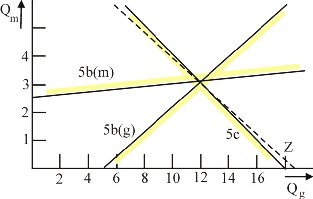
It has already been remarked that the problem can be solved by means of the graphical method. The graphical presentation uses the (Qg, Qm) coordinate space, where the inequalities 4b-d can be displayed as straight lines. The result is shown in the figure 1, using the assumptions, just mentioned (technique of table 1, etcetera).
In the figure 1 the solid black lines represent the boundaries of the inequalities 4b-d. The thick yellow strips are drawn simply to indicate the side of the boundary where solutions (Qg, Qm) for the pertinent inequality are allowed.
The line with the mark 5b(g) represents the inequality for the distribution of corn over the branches and over the nett product. In the same way the line with the mark 5b(m) represents the inequality for the distribution of metal. Both boundaries show that for the production of the desired nett product minimal quantities of corn and metal are necessary. The point of intersection of these two boundaries shows, that solutions are only possible past the point (Qg, Qm) = (12, 3.1).
The line with the mark 5c is the boundary due to the factor labour. This boundary shows that the quantity of available labour limits the size of the total product. The figure shows at one glance that in only a single point in the plane the three inequalities 4b-d are satisfied. This point is the common point of intersection, which has the values (Qg, Qm) = (12, 3.1).
In this point, which solves the problem, the surplus product is exactly equal to the desired nett product. The combined inequalities turn out to be simply equalities. Of course this result is not surprising, for this total product was once the starting point for the calculation of the technical coefficients. But still it is instructive to see the transformation of those equalities into the graph of the LP problem.
The question remains: what role is played by the target function in this LP problem? Since the problem is formulated in terms of the neoricardian price system, the target function must be redefined anyhow into Z' = Z/pg. Next choose the weighing factor, for instance pm/pg = 6.529. This is the price ratio, which corresponds to an efficiency of r=0.024. If desired the reader can check this in the figure 8 of the column, already mentioned, about the choice of the production technique. In this way the target function takes on the form Z' = 0.4745 × Qg + 1.026 × Qm. In the point (12, 3.1) the target function has the value 8.875/pg. It is evident (by definition) that this value equals the value of the desired nett product.
Apparently the target function in this problem is irrelevant. Since the inequalities have been reduced to equalities, there is no scarcity for any production factor. The available labour and the desired nett product are a perfect match for the current technique α. There is no need for an optimization.
Further in this column cases will be consirdered, where scarcity does occur, and thus optimization is required with regard to the production scale and perhaps with regard to the technique. Then it is convenient to conceive of the production function as a multitude of lines, who each represent a certain value Z'=c 9. In this manner the plane (Qg, Qm) can be covered with an infinite number of line functions, more or less like a map is covered with isotopes, which indicate the height. As an illustration the dotted line in the figure 1 represents the function line of all points, where the target function has the value c = 8.875. In mathematical terms this is Qm = 0.9747 × c − 0.4625 × Qg.
Needless to say, since there is no scarcity, the prices in this system can only be influenced by the conflict of distribution between the factors labour and capital. In other words, the markup for profit on top of the production costs determines the price ratios between the products.
In the neoclassical paradigm the subjective utility of a product fixes its price. According as the product is more scarce, the possession will be increasingly useful. The price is proportional to the marginal utility. That is to sayy, the price ratios are dictated by the ratios of the marginal utilities. In principle these prices are completely independent of the production costs10.
Such a situation can be created in the example, which has just been discussed, by the assumption that in future the producers must employ a quantity of labour L=32. That implies a growth of 6.67%. Suppose that the minimal consumptive demand on the market does not change and still equals QN = (3, 0.9). Then the LP problem of the set 4a-d becomes much more interesting. The figure 2 shows where in the new situation the boundaries are located.
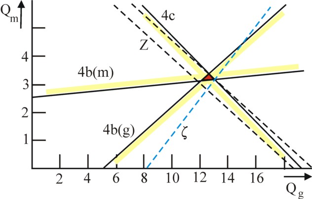
One sees how in the figure 2 the boundary corresponding to the inequality 4c in the (Qg, Qm) plane is shifted to the right. Thanks to the additional workers more can be produced than previously. The new surplus product exceeds the desired nett product. The red triangle in the figure 2 includes all total products Q, that are compatible with the desired nett product. Since the market demand QN no longer dictates the structure of the production in a unique manner, the question arises which surplus product is most desirable with regard to its size and structure.
It is known from mathematics, that the optimum will be located in an extreme of the possible area11. These are the angular points, namely (12.64, 3,389) and (13.10, 3.152), and obviously also (12, 3.1). Now the meaning of the target function becomes apparent. For she signals the preferences of the society. The needs will be satisfied best by the total product Q, that yields the largest Z value in one of the angular points. This problem can be solved in a graphical manner by shifting the function line as far as possible towards the right, without leaving the red triangle.
Pasinetti in his book points to the factor substitution, which according to the neoclassical paradigm must occur in such situations. The argument goes like this. Suppose that the weighing factors in Z is more or less neutral, for instance pm/pg = 1.5. The bale of corn and the ton of metal get approximately equal values. It turns out, that then the point (13.10, 3.152) yields the maximal rightward shift of the function line. That line is drawn in the figure 2, with the mark ζ, as blue dots12.
The growth rates of 9.17% and 1.68% show, that the agriculture has grown more than the industry. But in the neoclassical approach the physical quantities are not really relevant. The growth of the means of production must be related to the aggregated production capital, which is represented by the value of p·A·Q. After some computations one finds that in the optimal point the aggregated production capital has grown with 4.88%. That growth rate is smaller than the growth rate of L. In other words, thanks to the excessive quantity of labour the production technique has become more labour intensive, just as is predicted by the neoclassical paradigm!
At this point Pasinetti ends his arguments. That is unfortunate, because the present situation is really interesting. According to the neoricardian price theory the situation is actually quite complicated. For, the smallest price ratio for the technique α is 6.251, corresponding to an efficiency of r=0 (see again the column about the choice of the technique). For this price ratio the production line Z coincides exactly with the boundary 4c for the factor labour13. For all higher price ratios the function line will be flatter. In the figure 2 the function line is drawn for the case pm/pg = 6.529 (at r=0.024), as black dots, both for the starting point (12, 3.1) and for the new optimum. It turns out that for this type of price ratios the new optimum is located in the point (12.64, 3,389)! Here the exact value of the price ratio is not essential.
All growth efforts are directed towards the industry, while the nett product of the agriculture QgN remains unchanged. The situation is the reverse of the previous one. Now the optimum can not be explained in a simple manner. After some computations one finds that in the new optimum the aggregated production capital p·A·Q has increased by 8.22%. Despite of the excess of labour, the technique α has apparently become more capital intensive. That is a substitution, which conflicts with the intuitive expectations. Just now it became clear, that the high value of metal (pm/pg >> 1) is the direct cause. It can be added, that the growth occurs mainly in the industry, and she can employ the largest quantity of labour per unit of product.
In this maximum the target function Z obtains the value 9.47×pg. In the new optimum the surplus product is limited by the quantity of labour L=32. The other limiting factor is the minimal nett product QgN, which must at least be produced, because its creation requires capacity, which consequently is unavailable for the industry. Both L and QgN can be called resources. The production of metal benefits from a large quantity of L and from restrictions on QgN.
It is possible to calculate the rent prices π (also called shadow prices) of the resources (the nett product of corn QgN and metal QmN, and labour L), by means of the so-called dual LP problem. The shadow prices represent the marginal profit, which can be obtained from the addition of an extra unit of the pertinent resource14. Together they form a vector [πg, πm, πL]. The dual problem looks like this:
(6a) minimize Z = πg×QgN + πm×QmN + πL×L subject to the conditions
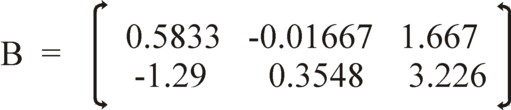
(6b) B · π ≥ p · (I − A)
The matrix B is the transposed matrix of the coefficients in the original LP problem 4b-c. In other words, B = [I−A†, a†], where † is the symbol for the transposition. That is to say, when the vertical vector [πg, πm] is represented by the symbol φ, then one has B · π = (I−A†) · φ + a†×πL. In order to avoid any misunderstanding the figure 3 displays the matrix B as a whole.
The interpretation of the target function 6a is that the costs of the chosen solution are minimal. The opportunity costs of other, not chosen, solutions are all higher.
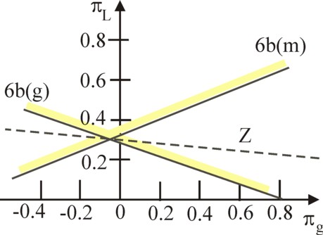
In principle an LP problem in three dimensions, such as the set 6a-b, can no longer be solved with the graphical approach. Actually the solution must now be calculated by means of the simplex method. But fortunately there is a way out. In the preceding text it has been explained that the nett product of tons of metal does not restrict the solution. In consequence, is does not make sense to decrease QmN. Therefore the corresponding shadow price πm will equal zero. This observation reduces the set 6a-b to merely the two dimensions (πg, πL).
The figure 4 shows where the boundaries in the dual problem are located. They intersect in the point pg × (-0.04461, 0.3). The allowed area consists of the "funnel" above the point. The "target value" line of the target function (Z=c) through this point is drawn as a dotted line. This minimum is found, when the lowest function line is identified, which just lies within the boundaries. Here the value c is pg × 9.47. This equals exactly the value, that is found for the target function of the primary LP problem. The agreement of the two Z values is a well-known hallmark of the primal and its dual15.
It is striking that the shadow price πg is negative. This means that the addition of a unit of QgN raises the costs. Conversely the abandonment of a unit of QgN results in a profit. Incidentally, your columnist has computed and checked the obtained solution (including πm=0) by means of the simplex method16.
It has just been announced that the prices of the available resources in the studied situation are no longer related to the production costs. The shadow price of a unit of QgN is independent of the "piece value", which is pg per bale. And the calculated wage level πL/pg = 0.3 deviates from the neoricardian wage level, which is πL/pg = 0.3 and can never be larger than 0.287 (the reader can verify this in the previous columns about the theory of Sraffa). All calculated shadow- (or rent-) prices are determined completely by the scarcity of the available resources. This is a fundamental difference with the situation in the previous paragraph.
The message in the text of Pasinetti can be summarized as follows: the neoricardian paradigm is not concerned with the problem of scarcity. When L increases with 6.67%, then according to the formula 5c the quantities Qg and Qm can be accordingly adapted without restrictions. If desired the structure of the nett product QN can be kept constant, by an increase of 6.67% for both Qg and Qm17.
On the other hand the neoclassical paradigm presupposes always a process of optimization. In this column the added value of the surplus product is maximized. Pasinetti stresses, that the optimization will commonly lead to a factor substitution, where the scarce production factors will be supplanted. Here Pasinetti refers to a switching of the technique. The present columns gives an illustration of the substitution process for pm=1.5, albeit only in the form of a price effect, and not as a concrete substitution.
Pasinetti states that the neoricardian mechanism is the normal manner for the (re-)establishment of the equilibrium of the economic system. As soon as scarcity occurs, the production capacity will be simply extended. In the short run the production factors can naturally be substituted, but that is not an equilibrium process. And prices can not be an indicator of scarcity. For as soon as labour is expended on a product, it must get a positive price, even when it is available in abundance.
Moreover, the column points to several nuances in the problem, which are not addressed by Pasinetti. This is unknown territory, so that mistakes can not be excluded. The column supplements the arguments of Pasinetti with the observation, that the price system can interfere with the neoclassical mechanism of substitution. There is the price effect that for pm/pg = 6.529 the production turns out to become more capital intensive, even though the factor labour is present in abundance. Also it is shown that with regard to the physical characteristics of the production, a shift towards more labour-intensive activities does occur (notably the industry). It is well known, among others thanks to the phenomenon of reswitching, that prices and substitution do not influence each other in a monotonous way.
Another supplement with regard to the book of Pasinetti is the discussion concerning the stability of the weighing factor(s) in the target function 4a. A part of the surplus product is allocated to the desired nett product, in order to guarantee minimal consumer requirements. No statement is made about the distribution of the remainder of the surplus product, after the optimization of its value. Suppose that the extra metal is available for raising the wage. The increased supply of metal will probably incite the wage-earners to reduce their marginal utility of metal. Metal can not be digested. Then the original price pm is no longer sustainable, at least if markets must be cleared. But a changing pm will undermine the whole optimization procedure.
In an alternative scenario the extra metal can be paid as a profit to the entrepreneurs. In that case the maximization of the added value is simply an optimization of the profit. Tons of metal are a convenient savings (as long as they do not rust). Perhaps thus the marginal utility of metal is fairly stable for the entrepreneurs, as log as the price pm is maintained in spite of the optimization. This reminds somewhat of the Leninist rule of thumb, that the total utility is approximately proportional to the quantities.
It would be interesting to study also the situation, where the various branches can choose between different methods of production. What would happen with the level of activity of each producer, when for instance the employment is raised somewhat? Evidently the real effects are more exciting than merely the price effects. It is clear that this more complex problem can only be studied by means of the simplex method. This exercise will be postponed to a future column.