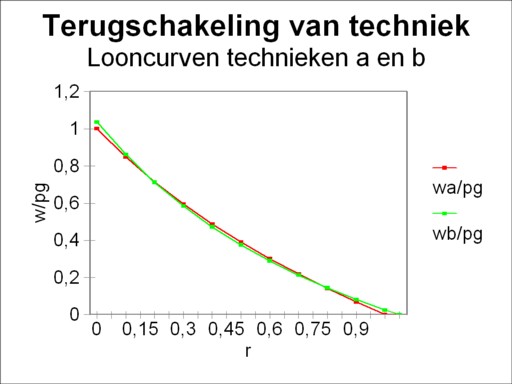
Figure 1: Wage curves for α and β
In the neoricardian theory of Piero Sraffa it is shown that there is no evident relation between the distribution of income (wage and profit) and the choice of the technique for production. It is even conceivable that with the progress of time subsequent switches between two techniques occur (the so-called reswitching). In this way Sraffa undermines several fundamental assumptions of the neoclassical (marginalistic) macro-economics. For she relies on factor substitution: in case of for instance a rising rate of interest the factor capital in the production process will be replaced by the factor labour. The phenomenon of the reswitching of techniques illustrates that such a monotonous trajectory of substitution is not inevitable.
If one wants to understand the macro-economic developments, then the analysis of the economic structure is unavoidable. The composition of the total social product and its method of production are essential for the behaviour of the prices, the wages and the profit. Therefore this portal has on several occasions drawn attention to the neoricardian theory of Sraffa. Recently a column has explained how the producers choose their production technique. In that column the future discussion of the so-called reswitching phenomenon has been announced. The present column redeems that promise.
For the benefit of those readers, who have not read the preceding column(s), a succint description of the neoricardian formalism will again be presented. However, persons who are not familiar with this theory, are well advised to consult first the previous columns about the subject. Those who are really fascinated by the matter, can consult the original sources, that have been used by your columnist. The formalism is explained in the excellent book Vorlesungen zur Theorie der Produktion by the famous economist Luigi L. Pasinetti1.
In the theory of Sraffa the producer j receives for his production a proceeds given by the formula
(1) pj × Qj = (1 + r) × Σi=1n (pi × qij) + w × lj
In the formula 1 the time dependency is ignored, such as during economic growth. The quantity Qj is the material yield of the producer j, qij is the amount of product i that is used for the production of j, and lj is the expended amount of labour. There is a total of n producers in the system, with each a different end product, so that the summation runs from 1 to n. The variable pi represents the price of product i, and w is the wage level.
The efficiency r of capital can be interpreted as the rate of profit, that is common in the existing social conditions. The interest must be paid from the profit. When it is assumed that the producers obtain little profit, then r equals the rate of interest. Apparently there are n+2 unknown variables, including the efficiency r. The calculation of those variables becomes more transparent, when the quantities are removed from the formula 1. The division of the left- and righthand part by Qj yields
(2) pj = (1 + r) × Σi=1n (pi × aij) + w × aj
In the formula 2 aij = qij / Qj are the production coefficients, and aj = lj / Qj is the labour coefficient. The n+1 components of the column [aij, aj], which characterizes the production process, are called the technical coefficients. Together they describe the technique of the production process. The advantage of the form in the formula 2 becomes clear, when the absence of scale effects is assumed. When the production on a larger scale does not yield positive or negative returns, then the quantities of the used production factors per unit of product remain unchanged. Then the technical production coefficients are constants, and the formula 2 is a linear equation.
The producer j can not solve the formula 2 by himself. He must accept that the market fixes the prices of the raw materials and of the equipment. The solution is only possible at the macro-economic level, where the formula 2 is a vector equation:
(3) p = (1 + r) × p · A + w × a
The matrix A has the dimension n×n and is composed of the production coefficients. Obviously here the vectors p and a are horizontal, so 1×n.
Thanks to the matrix calculation the formula 3 can be solved simply for p. One finds
(4) p(r) = w × a · (I − (1 + r) × A)-1
In the formula 4 I is the unity matrix. The upper index -1 indicates, that the inverse of the matrix between the two brackets must be taken. If desired the reader can find an application of this formula in a previous column. This theory shows clearly how the knowledge from mathematics can contribute to the economic insights. The reader can consult the annex (below the footnotes) for some typical features of the mathematics of Sraffa.
Since the set of n equations can not determine n+2 variables, it is common to choose a numéraire. The wage level w is an obvious choice for this. This results in n+1 unknown variables, namely r and n ratios pj/w. In other words, since only n equations are available, the pj/w functions will depend on r.
When the price functions are inverted, then the variables change into (w/pj)(r). These variables are called wage curves, each one related to a certain price pj. In other words, there are n different wage curves. The collection of wage curves is characteristic for the corresponding production technique. In this column it is assumed that the branch (group of firms with the same product) with j=1 produces corn. Henceforth only the wage curve (w/pg)(r) will be studied.
When w/pg is expressed in prices, then they will take on the form p/pg 2. Apparently the focus on the wage curve w/pg implies, that in fact the price pg of a bale of corn becomes the new numéraire, which is indeed rather arbitrary. Incidentally any choice from the collection of wage curves would have sufficed, because in general one is only interested in the ratios of the prices. The numéraire drops out in those ratios.
Producers try to minimize their costs. In the column about the choice of the production technique it is shown, that therefore the producers tend to prefer the production technique, which defines the technology frontier. The technology frontier is the envelope of all available wage curves. According as more techniques γ become available, the number of possible wage curves increases. In this way the technology frontier will probably extend and expand. Thus for a given capital efficiency r the producers prefer the technique α, which yields the heighest wage level (w/pg)(r). In the following text the wage level which belongs to the technique α will be denoted by (w/pg)α. So here the upper index α does not represent an exponent.
The role of the wage curves in the choice of the technology is naturally not really surprising. The highest wage level w/pg for a given r is identical to the heighest nett product for that value of r. And a large nett product offers extra room for profit. Indeed the preceding text can also be interpreted in such a way, that for a given wage level the technology frontier yields the largest rate of profit r.
The neoricardian theory shows that in a complex economic system with many branches each wage curve is a complex polynomial in r. Therefore the wage curve as a function of r exhibits an undulatory motion, although she also descends in a monotonous manner. In other words, the rising capital efficiency r is paid by means of a lower wage level. Due to the undulating behaviour the wage curve of each technique may at some point determine the technology frontier. The reader can again consult the annex below the footnotes for the mathematical peculiarities.
Such a complicated technology frontier is not very suited for a simple analysis. Since the present column aims to illustrate the phenomenon of the reswitching of a technique, it suffices to consider an economic system with only two branches.
These columns rarely mention the time that is needed for their completion. For this study of reswitching your columnist must admit, that the construction of an example required at least ten working-days. Is this worth the effort, considering the alternative option of simply copying an example from text books?3 Was this time spent on scribbling formulas better invested in making fun with people? Even more so, since that yields a social reward? Yet your columnist does not think so. Thanks to the theory of reswitching large parts of the neoclassical macro-economics can be abolished. That is such an essential feat of arms, that a lover of economics really has to master the reswitching model.
A good alternative would have been to use the construction method for reswitching situations, which is presented in the paper Creating two-good reswitching examples by Robert Vienneau. Vienneau is a dedicated adherent and expert of the neoricardian theory. Unfortunately your columnist discovered this paper only a couple of days ago. At that time he had already invented his own approach. Incidentally the method of Vienneau was a stimulus in order to perfect the approach. Therefore the link to the paper is warmly recommended to readers who are truly interested4. In addition the book The production of commodities by J.E. Woods deserves mentioning, because it has led the way for the construction of the following example5.
An economic system with only two branches is considered, namely the agriculture for the production of corn (in bales) and the industry for the production of metal (in tons of weight). Here the loyal reader recognizes the examples from preceding columns. In the two branches the relevant economic variables are supplied with respectively the indexes g and m. When the formula 4 is written out in detail, then one finds6
(5a) (w/pg)(r) = (1 − Σ × (1+r) + Δ × (1+r)²) / ( ag − Ψ × (1+r))
(5b) Σ = agg + amm
(5c) Δ = agg × amm − amg × agm
(5d) Ψ = amm × ag − amg × am
People with some knowledge of matrix calculations will recognize in Σ the trace of the matrix A, and in Δ the determinant of A. It turns out that the numerator of the wage curve is a polynomial of degree 2 in r. The first intersection of the polynomial represents the situation, where the whole nett product is paid as a profit. Beyond that point the set of equations 5 is not relevant for the economy, nor the domain r<0 either. Now the reader will perhaps understand, why the construction of a wage curve is so complicated, and thus imposes such a heavy burden upon your columnist7.
The wage curve of the set 5 is valid for a single technique. Reswitching requires at least two techniques. Suppose that the agriculture only disposes of the production method τ(g1). Suppose on the other hand that the industry can choose from two production methods, namely τ(m1) and τ(m2). The table 1 displays the values of the technical coefficients for these three methods, that will be used in the present exemple. The index j is either g or m, corresponding to respectively the agriculture- or industry column in the table. Apparently at the macro economic level there exist two techniques, each consisting of a combination of the two methods at the level of the branch (namely agriculture and industry). Here the techniques are called α = (τ(g1), τ(m1)) and β = (τ(g1), τ(m2)). In other words, each technique consists of a combination [Aθ, aθ], with θ = α or β.
| agriculture | industry | ||
|---|---|---|---|
| τ(g1) | τ(m1) | τ(m2) | |
| agj | 0.07 | 0.4042 | 0.06588 |
| amj | 0.5 | 0.03 | 0.41 |
| aj | 0.05 | 1.303 | 0.9362 |
The table 1 shows that the choice for a (re-)switch in the industrial production method changes the proportions of the production factors. It is obvious that per ton of used metal the production technique τ(m1) uses a relatively large amount of corn and the production method τ(m2) uses a relatively large amount of metal.
Now that the technical coefficients have been fixed, the two wage curves (w/pg)α and (w/pg)β can be expressed in a mathematical manner by means of the set 5a-d8. Subsequently the numerical values of both wage curves can be calculated. The result of these calculations is presented in the figure 1. For the general explanation of the meaning of the wage curves the reader can consult the previous column about the choice of the technique. The wage curves in the figure 1 are special, because they intersect twice: in the points r=0.2 and r=0.8.
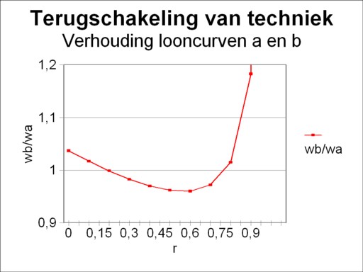
Perhaps this phenomenon is difficult to see, because for this simple case the two wage curves remain very similar in shape. The phenomenon is better observable in the figure 2, where for each r the ratio of the value (w/pg)β(r) with respect to the value (w/pg)α(r) is depicted. In the r-domain [0, 0.2] the technology frontier is determined by the technique β, and subsequently in [0.2, 0.8] by the technique α, and finally in [0.8, 1.05] again by the technique β.
The switching of the technique β to the technique α and then back again to the technique β is a conscious choice of the producers in the industry. This example illustrates that a raise of the capital efficiency r does not naturally favour one technique over the other. There are no rules of thumb for the switching, in the way that is suggested by the neoclassical paradigm. Apparently the specific structure of the total production is decisive in the decision-making.
In the preceding column about the choice of the technique it has already been stated, that the changes of the economic variables during a raise of the capital efficiency r are not always real. Sometimes they are just a price effect. For instance the value of the means of production can rise, even when in reality the technique remains identical, simply due to the development of the prices. A real effect occurs when the producers make the concrete and conscious decision to prefer another production method. The table 1 shows, that such a decision changes the quantities of the production factors (material and labour) per produced unit of the end product.
Quite surprising is the development of the factor labour. First, it is striking that apparently the labour productivity (represented by Qm/lm, the inverse of the labour coefficient am) is higher for the method τ(m2) than for the method τ(m1). However, this difference is not very important, because the producers are interested mainly in the nett product. A high labour productivity, which is transformed mainly into the replacement of the worn-out means of production, would not give them much (added) value.
Obviously, it is interesting to study the reactions of the producers to a falling wage level. The switch from τ(m1) to τ(m2) in the first switching point (at r=0.2) shows that despite the falling wage level the producers prefer a method, which requires less labour per ton of metal. At first sight this does not appear to be a logical choice, and so it is an anomaly. The reswitching at r=0.8 does appear a sensible choice, and confirms the intuitive feeling.
The development of the means of production is more complicated. For a clear understanding it is necessary to compute the development of the prices of the materials. In a similar way as for the set of equations 5a-d the price ratios can be calculated9
(6a) (pm/pg)(r) = (ag − Φ × (1+r)) / ( ag − Ψ × (1+r))
(6b) Φ = agg × am − agm × ag
In the formula 6a Ψ has the same meaning as in the formula 5d.
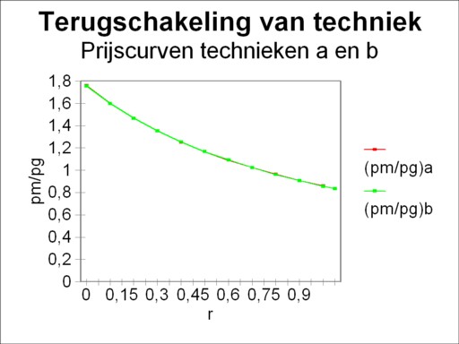
The two price ratios (pm/pg)α and (pm/pg)β can be written in a mathematical way by means of the set 6a-b10. Next the numerical values of both curves can be computed. The result of these computations is shown in the figure 3. The two price curves for the techniques α and β turn out to be almost equal in the considered domain of r-values. Thus it remains invisible, that in the switching points both techniques yield exactly the same prices.
However, more important is that a raise of the capital efficiency is accompanied by a significant fall of the price pm of a ton of metal with respect to the price pg of a bale of corn. Incidentally, this monotonous pattern of changing prices (∂/∂r(pm/pg) < 0) is the hallmark for all techniques with a convex wage curve. In view of this behaviour of the prices, which is obervable for the producers, it is intuitively strange that at the second switching point (r=0.8) the producers prefer the production method, which per ton of newly produced metal uses more corn and less metal. This is again an anomaly. The choice of the producers at the first switching point (r=0.2) does make sense, because here the situation is the reverse.
It has already been stated in the previous column about the choice of technique, that during reswitching the occurrence of anomalies is unavoidable. For reswitching implicates that the producers follow an oscillating policy. It is this deviation from the monotonous behaviour, which destroys the foundation of several hypotheses in the neoclassical macro-economics.
Thanks to mathematics it is possible to describe how the capital efficiency r and the wage level w influence each other and the product prices. The economic system is transformed into a mathematical model. One must be well aware that the economic principles impose constraints on the possible mathematical solutions. For instance mathematics does not object to negative prices, but the economy does. This annex is based mainly on the book Vorlesungen zur Theorie der Produktion by L.L. Pasinetti. At several places your columnist adds his own elaborations.
It is at least for people with a mathematical affinity interesting and enlightening to analyze what exactly the set 5 implies with respect to the behaviour of the wage level (w/pg)(r). That wage level is expressed in the prices p(r), which in turn are fixed by the formula 4. In the formula 4 the inverse of the matrix (I − (1 + r) × A) appears, where the elements depend on r in a linear way. When the inverse matrix is calculated, then a division by the determinant of (I − (1 + r) × A) is required. The reader can verify this in any book about linear algebra and matrix calculations, or consult a previous column about the theory of Sraffa. In other words, the prices are inversely proportional to the determinant of the matrix. In this case the matrix elements are proportional to r, and thus the determinant is a polynomial of degree n in r. Therefore the prices have a polynomial of degree n in r as the denominator. Since in the wage curve the wage level w is divided by a price, in this case pg, that polynomial of degree n turns up in the numerator.
A polynomial of degree n has at most n zero points. Thus this is also true for the wage level (w/pg)(r). Such a behaviour of the wage level is strange from the economic point of view. For in the first zero point w/pg(r1) = 0 the whole nett product is paid as profit. Then the wage level can not be positive for an even larger value of r. That is to say, from the economic point of view the formulas 4 and 5 are not usable for values of r past the first zero point r=r1. It can be proven by means of mathematics, that above that zero point the formula 4 leads to negative values for some prices. See p.98 and p.290 and further in the book of Pasinetti. It is obvious that one must be well aware of this restriction.
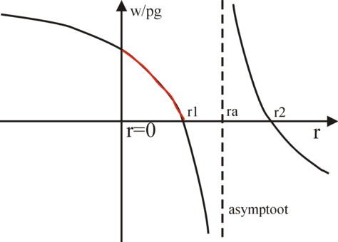
Figure 4: Mathematical wage curve
with asymptote and two intersections
It has already been remarked in the main text of this column that the mathematical model yields a the wage curve, which in the domain of valid values of r falls in a monotonous manner. The monotonous decrease has an oscillating shape, in accordance with the characteristices of the polynomial in r. See p.108 and p.296 in the book of Pasinetti.
The example with two branches, and thus with a dimension n=2, provides for a fascinating illustration of the mathematical form of the wage curve. In the case n=2 the numerator consists of a polynomial of degree 2, which has two zero points r1 and r2. However, the denominator of w/pg contains a linear function of r. This function does not cause problems until the first zero point r1, but past r1 she leads to an asymptotic behaviour at r=ra. This phenomenon is shown in a graphic manner in the figure 4.
In the figure 4 the asymptote r=ra divides the domain of r-values in two parts. On the left-hand side the wage curve is concave (bulging away from the axis), and on the right-hand side she is convex (bulging towards the axis). When ra of the asymptote has a positive value, then the wage curve is concave in the domain of r-values, that is economically relevant. Then the asymptote lies past r1 of the first zero point. That is the situation of the figure 4. When ra of the asymptote has a negative value, then the wage curve is convex in the economically relevant domain of r-values.
The actual behaviour depends naturally on the coefficients in the linear set of the formula 4. In other words, the chosen production technique determines the location of the asymptote. A change of technique can shift the wage curve in any direction. Your columnist has played a little with the set 5 in order to construct a case of reswitching, that has a concave and a convex wage curve. This attempt has failed. Indeed according to the no reswitching theorem that situation is impossible, at least for the case with n=2. See p.87 and further of The production of commodities. But in more complicated situations, with three or more techniques, such cases do occur.